Statistical Inference Concerning Local Dependence between Two Multinomial Populations

2003, Vol. 14, No.2 pp. 413∼428

Statistical Inference Concerning Local Dependence between Two Multinomial Populations

Myongsik Oh¹⁾

Abstract

If a restriction is imposed only to a (proper) subset of parameters of interest, we call it a local restriction. Statistical inference under a local restriction in multinomial setting is studied. The maximum likelihood estimation under a local restriction and likelihood ratio tests for and against a local restriction are discussed. A real data is analyzed for illustrative purpose.

Keywords : Chi-bar-square, local dependence, likelihood ratio ordering, stochastic ordering, uniform stochastic ordering.

1. Introduction

In statistical analysis of 2×k contingency table, the most frequently used statistical concept is dependence. This dependence concept is closely related to various types of stochastic ordering, such as usual stochastic ordering, uniform stochastic ordering (hazard rate ordering for continuous random variables), likelihood ratio ordering and dominated ordering, among others. Douglas, Fienberg, Lee, Sampson, and Whitaker (1990) provides an excellent illustration of these relationships. Statistical inference under such ordering have been studied by many researchers. Robertson and Wright (1981) studied statistical inference concerning stochastic ordering between two multinomial populations, Dykstra, Kochar, and Robertson (1991, 1995) provided statistical inferential procedure for uniform stochastic ordering and likelihood ratio ordering. Park, Lee, and Robertson (1998) studied likelihood ratio test for uniform stochastic ordering in two or more discrete distribution with the same support. Chang (1993) studied dominance ordering for 1) Associate Professor, Department of Statistics, Pusan University of Foreign Studies,

Busan, 608-730, Korea

E-mail : [email protected]

two multinomial parameters.

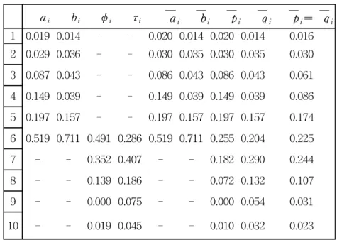
We consider the following example which has motivated of this study. In the academic years of 1997 and 1998, 280 and 208 students were admitted to the College of Oriental Studies, Pusan University of Foreign Studies respectively. For each academic year stdents were classified into 10 groups according to their high school ranks. There are originally 15 scales in high school ranks but only top 10 scales are used. The smaller the number, the higher the school rank. It is well known that the academic performance of first year college students is closely related to their high school ranks. The higher the school rank, the better GPA in the first year. A school official claims that for high school rank 5 or above the portion of admitted students up to certain high school rank has increased in 1998 compared to 1997. Let pi the proportions of ith group for admitted students in 1998 and q _i be the proportions of ith group for admitted students in 1997. Then the school official's assertion may be hypothesized as a local stochastic ordering, i.e., ∑

i

j = 1p_j≥∑

i

j = 1q_j for i = 1,…,5. We are interested in testing

H ₀:p _i= q _i for i = 1,…,10 versus H₁:∑

i

j = 1p_j≥∑

i

j = 1q_j for i = 1,…,5.

We call this type of restriction local dependence. As we discussed before there are several types of dependence. First suppose local odds ratios, piq _{i + 1}/p _{i + 1}q _i, are greater than or equal to 1 for i= 1, …,k0. This is equivalent to that p i/q _i is nondecreasing in i= 1, …,k₀, which shows likelihood ratio ordering locally.

Second, suppose p _i ∑^k

ℓ = i + 1q_ℓ/q _i ∑^k

ℓ = i + 1p_ℓ≥1 for i = 1, …,k 0. It is equivalent to that ( 1 - ∑ⁱ

ℓ = 1p_ℓ)/( 1 - ∑ⁱ

ℓ = 1q_ℓ) is nonincreasing in i = 1, …,k₀, which shows uniform stochastic ordering locally. Third, suppose

∑ⁱ

ℓ = 1p _ℓ ∑^k

ℓ = i + 1q_ℓ/ ∑ⁱ

ℓ = 1q_ℓ ∑^k

ℓ = i + 1p_ℓ≥1 for i = 1, …,k 0. This is equivalent to

∑

i

ℓ = 1p _ℓ≥ ∑

i

ℓ = 1q_ℓ for i = 1, …,k ₀, which is similar to stochastic ordering locally. Finally, let p_i≥q _i for i = 1, …,k ₀, which is similar to dominated ordering locally. It is appropriate to use the term ``local" in front of each ordering since the transformations of parameter preserve the corresponding ordering as we will see later.

In this paper we are going to discuss the statistical inferences when one of four types of local dependence is imposed to a 2×k contingency table. In Section 2, maximum likelihood (ML) estimate of cell probabilities under the local dependence restriction is discussed. Transformation of parameter space is required to find cell

probabilities. In section 3, likelihood ratio tests (LRT's) of equality of two parameter against local dependence is studied. The asymptotic null distributions of test statistics are derived.

2. Estimation

In this section we are going to investigate the estimation procedure for four types of local dependence restrictions. For each type of restriction, the key step is reparametrization of parameter space before applying the existing estimation procedure. However the reparametrization scheme for each restriction is different from ordering to ordering.

Let p = ( p ₁,p ₂,…,p _k) and q = ( q ₁,q ₂,…,q _k) be the probability vectors.

Suppose that p and q are the relative frequencies of successes corresponding to independent random samples of sizes m and n from the p and q populations, respectively. Let N=m+n and let p and q be the ML estimates of p and q, respectively. Note that we use the same notation for restricted ML estimate regardless of restriction type unless it causes confusion.

2.1 Local stochastic ordering

Suppose ∑ⁱ

j = 1p_j≥ ∑ⁱ

j = 1q _j for i = 1, …, k₀. Let a _i= p_i, b_i= q_i for i = 1, …,k₀, a _{k0+ 1}= ∑

k

j = k0+ 1p_j, b _{k0+ 1}= ∑

k j = k0+ 1q _j, φ _i= p _i/a _{k0+ 1}, τ _i= q _i/b _{k0+ 1} for i = k₀+ 1, …,k. Then the basic restriction

becomes ∑

k0+ 1

i = 1 a _i= 1, ∑

k0+ 1

i = 1 b_i= 1, ∑^k

i = k0+ 1φ _i= 1, ∑^k

i = k0+ 1τ_i= 1 and 0 < a _i,b _i, φ_i, τ _i< 1. The local stochastic ordering restriction becomes

(2.1)

∑ⁱ

j = 1a_j≥∑ⁱ

j = 1b_j for i = 1,…,k₀, and ∑

k0+1

j = 1 a_j= ∑

k0+1 j = 1 b_j. The likelihood function becomes

(2.2)

[^{∏i= 1k0am pi i⋅a ∑}

k

j = k0+1m pj

k0+1 ⋅∏

k0

i= 1b^{n q}_i ⁱ⋅b ^∑

k

j = k0+1n qj

k0+1 ]^⋅[^{i = k∏k0+1φm pj jτn qj j}]^.

We observe that no restrictions except (2.1) relate a _i, b _i, φ_i and τ _i to each other. The maximum of (2.2) under (2.1) is obtained by maximizing the two parts (each in bracket) separately.

First consider the latter part in (2.2). Since no restriction other than basic

restrictions are imposed each is just a usual multinomial model and hence φ _i= φ _i= m _i/ ∑^k

j = k0+ 1m _j and τ_i= τ _i= n _i/ ∑^k

j = k0+ 1n _j, for i = k ₀+ 1, …,k. For the first part we can use estimation procedure in Robertson and Wright (1981). The restricted are given by

a = a E _a

(

)

b = b E _b

(

)

)

where A = { x ∈ R ^{k0+ 1}:x₁≥x₂≥…≥x_{k0+ 1}}, I = { x ∈ R ^{k0+ 1}: - x ∈ A }, and all vector operations are componentwise. Evaluation of p and q at a = a, b = b , φ _i= φ _i, τ_i= τ_i for i = k ₀+ 1, …,k gives the restricted ML estimates p and q.

Suppose p = q. This is equivalent to a_i= b_i for i = 1,…,k ₀+ 1 and φ _i= τ_i for i = k₀+ 1, …,k. Then the ML estimates under this restriction are given by

a _i= b _i= m p _i+ n q _i

N , for i = i = 1, …,k ₀, a _{k0+ 1}= b _{k0+ 1}=

m ∑^k

j = k0+ 1 p_i+ n ∑^k

j = k0+ 1 q_i

N ,

φ _i= τ _i= m p _j+ n q _j

∑^k

j = k0+ 1(m p _j+ n q _j)

, for i = k₀+ 1, …,k.

2.2 Local uniform stochastic ordering

Suppose ( 1 - ∑ⁱ

ℓ = 1p_ℓ)/( 1 - ∑ⁱ

ℓ = 1q_ℓ) is nonincreasing in i = 1, …,k 0. For this restriction we don't need another transformation of parameter space other than the transformation used for the case k ₀= k. Let θ _1j= ∑^k

ℓ = j + 1p _ℓ/ ∑^k

ℓ = jp_ℓ and θ _2j= ∑^k

ℓ = j + 1q_ℓ/ ∑^k

ℓ = jq_ℓ for j = 1,…,k - 1. Then p₁= 1 -θ₁₁,

p_j= (1- θ_1j) ∏

j - 1

ℓ = 1θ _1ℓ for j = 2, …, k - 1, p_k= ∏

k - 1

ℓ = 1θ _1ℓ, q₁= 1 -θ₂₁, q_j= (1- θ_2j) ∏^{j - 1}

ℓ = 1θ _2ℓ for j = 2, …, k - 1, q_k= ∏^{k - 1}

ℓ = 1θ _2ℓ. Since

∑

k

ℓ = jp _ℓ= ∏

j - 1

ℓ = 1θ _1ℓ, ∑

k

ℓ = jq_ℓ= ∏

j - 1

ℓ = 1θ _2ℓ for j = 2,…,k, the restriction becomes (2.3) θ_1j≤θ _2j for j = 1,…,k₀-1

and the likelihood function is

(2.4)

∏

k - 1 j = 1[^{θ ∑}

k

ℓ = j + 1m pℓ

1j (1-θ_1j)^{m pj}⋅θ ^∑

k

ℓ = j + 1n qℓ

2j (1-θ_2j)^{n qj}]^.

Note that for j = k ₀, …,k - 1 no restriction is imposed between θ _1j and θ _2j. The basic restriction is 0 <θ_ij< 1 for i = 1, 2, j = 1, …, k - 1. Since the restriction does not relate θij for different j, the maximum of (2.4) under (2.3) can be achieved by maximizing j-1 terms (each in bracket) separately. Then restricted ML estimates are

θ _1j= θ_1j, θ _2j= θ _2j if θ_1j≤ θ _2j, for j = 1, …,k ₀- 1, θ _1j= θ _2j= θ_1j= θ_2j if θ _1j> θ_2j, for j = 1, …,k ₀- 1, θ _1j= θ _1j, θ _2j= θ _2j, for j = k ₀, …,k - 1,

where for j = 1,…,k - 1,

θ _1j= θ _2j=

m ∑^k

ℓ = j + 1 p_ℓ+ n ∑^k

ℓ = j + 1 q_ℓ m ∑^k

ℓ = j p _ℓ+ n ∑^k

ℓ = j q_ℓ .

Evaluation of p and q at θ _ij= θ_ij for i = 1, 2 and j = 1,…,k - 1 gives the restricted ML estimates p and q. The ML estimate of θ _ij under restriction

p = q is θ_ij.

2.3 Local likelihood ratio ordering

Suppose p_i/q _i is nondecreasing in i = 1, …,k ₀. Let a _k0= ∑

k0

i = 1p _i, b _k0= ∑

k0

i = 1q _i and ai= p _i, b_i= q _i for i = k 0+ 1, …,k. Let θ _i= m ^'p_i/a _k0

m ^'p_i/a _k0+n^'q_i/b_k0 , φ _i= m ^'p_i/a _k0+ n ^'q _i/b_k0 for i = 1, …, k ₀, where m^'= m ∑

k0

i= 1p_i and n ^'= n∑

k0

i= 1q_i. The basic restrictions become (1) 0 <a _i, b _i< 1 for i = k ₀, …,k, (2) ∑

k i = k0

a _i= ∑

k i = k0

b_i= 1, (3) 0≤θ i≤1, φ_i≥0 for i = 1,…,k ₀, (4) ∑

k0

i= 1φ _i= m ^'+ n ^', and (5)

∑

k0

i= 1θ _iφ _i= m ^'.

The local likelihood ratio ordering is equivalent to

(2.5) θ ₁≤…≤θ_k0.

The likelihood function is proportional to

(2.6)

[^{i= 1∏k0θm pi i(1-θi)n qiφm pi i+n qi}]^⋅[^{amk0'bnk'0i = k∏k0+1am pi ibn qi i}]^.

Since the restrictions together with basic restrictions do not relate the first and second parts (each in bracket), the maximum of (2.6) can be obtained by maximizing two parts separately. The maximization of the second part is easy and hence we have a _k0= m ^'/m , b_k0= n ^'/n, and a _i= p _i, b_i= q _i for

i = k ₀+ 1, …,k.

The maximization of the first part is little bit complicated. The whole procedure is well described in Dykstra et al. (1995). Let φ _i= m p _i+ n q _i for

i = 1,…,k ₀ and let θ = E _w( θ |I ) where

w = ( m p ₁+ n q₁, …,m p _k0+ n q _k0). Then it follows from Theorem 1.3.3 of Robertson et al. (1988) that ∑

k0

i= 1 θ _i φ _i= m ^' and hence maximize (2.6) under (2.5) with basic restrictions. Evaluation of p and q at θ _i= θ _i, φ_i= φ_i for j = 1,…,k - 1, and a_i= a _i, b_i= b _i for i = k 0, …,k gives the restricted ML estimates p and q.

Suppose p = q. Then p_i= q_i= (m p _i+ n q_i)/(m+ m) for i = 1, …, k.

We have a _k0= b _k0= (m^'+ n ^')/(m + n),

a _i= b _i= (m p _i+ n q _i)/(m + m) for i = k₀+ 1, …,k, and θ _i= m ^'/(m^'+ n ^'), φ _i= (m p_i+ n q_i) for i = 1, …,k ₀.

2.4 Local dominated ordering

Suppose pi≥q _i for i = 1,…,k ₀. Let a i= p _i, b i= q_i for i= 1, …,k 0 and a _{k0+ 1}= ∑^k

j = k0+ 1p_j, b _{k0+ 1}= ∑^k

j = k0+ 1q _j. Let θi= p _i/a _{k0+ 1} and η i= q _i/b _{k0+ 1} for i = k₀+ 1, …,k. Then the basic restriction become (1) 0≤a _i, b_i≤1 for

i = 1,…,k ₀+ 1, (2) ∑

k0+ 1

i = 1 a _i= ∑

k0+ 1

i = 1 b_i= 1, (3) 0≤θ_i, η _i≤1 for

i = k ₀+ 1, …,k, and (4) ∑

k

i = k0+ 1θ _i= ∑

k

i = k0+ 1η_i= 1. The local restriction becomes (2.7) a_i≥b_i for i = 1,…,k₀

The likelihood function is proportional to

(2.8)

[^{∏i= 1k0am pi ibn qi iam ∑}

k

ℓ = k0+1pℓ

k0+1 b

n ∑

k

ℓ = k0+1qℓ

k0+1 ]^⋅[^{i = k∏k0+1θm pi iηn qi i}]^.

No restrictions relate the two parts (each in bracket) in (2.8) to each other and hence (2.8) can be maximized by maximizing two parts separately. From the second part we have θ _i= θ_i= m p _i/m ^', η _i= η _i= n q_i/n ^' for

i = k ₀+ 1, …,k, where m^'= m ∑^k

i = k0+ 1 p_i and n ^'= n ∑^k

i = k0+ 1 q_i.

For the first part, Fenchel dual plays a fundamental role in estimation of restricted ML estimate of a = ( a ₁, …,a _{k0+ 1}) and b = ( b ₁, …,b _{k0+ 1}). The rigorous estimation procedure for the case of k 0= k is given in Chang (1993).

However we briefly state the estimation procedure here. Let T = { x ∈ R ^{k0+ 1}:x_i≥x_k, i = 1,…,k ₀}. Then the Fenchel dual of T, denoted by T ^{w *}, is given by

{ x ∈ R ^{k0+ 1}:w_ix_i≤0, i = 1,…,k₀, ∑

k0+ 1

i = 1 w_ix_i= 0 }.

We also note that it follows from mathematical induction that

(2.9) a _i≥ m a_i+ n b _i

N ≥ b_i for i = 1,…,k₀. Let B be defined by

{ u ∈ R ^{2k0+ 2}:u_i≥u_{k0+ 1} for i = 1,…,k₀, and u_i≤u_{2k0+ 2} for i = k ₀+ 2, …,2k ₀+ 1 }.

Let

h _i = N ^{- 1}+ n mN

a _i

b_i , i = 1,…,k ₀+ 1,

= N ^{- 1}+ m nN

a _{i - k0- 1}

b_{i - k0- 1} , i = k ₀+ 2, …,2k₀+ 2, w = ( m a ₁, …,m a _{k0+ 1}, n b ₁, …,n b _{k0+ 1}),

t = ( a ₁/m a ₁, …,a _{k0+ 1}/m a _{k0+ 1}, b ₁/n b ₁, …,b _{k0+ 1}/n b _{k0+ 1}).

Then restriction (2.9) together with basic restriction become

(2.10) ( t_i-h_i)w_i≥0 for i = 1,…,k₀,

( t_i-h_i)w_i≤0 for i = k₀+2, …,2k₀+1, and

∑

k0+1

i = 1(t_i-h_i)w_i= ∑

2k0+2

i = k0+2(t_i-h_i)w_i= 0.

Restriction (2.10) can be rewritten as h - t ∈B^{w *}. Hence

t = ( a ₁/m a ₁, …, a _{k0+ 1}/m a _{k0+ 1}, b ₁/n b ₁, …, b_{k0+ 1}/n b _{k0+ 1}) solves

minimize ∑

2k0+ 2

i = 1 w_if(t_i) subject to h - t ∈B^{w *}.

Appealing to Theorem 3.4 of Barlow and Brunk (1972), we have ( a , b ) = w E _w( h |B). Since membership in B imposes no restriction between the first k₀+ 1 coordinates and the last k₀+ 1 coordinates of a point, ( E( ⋅|B)₁, …,E( ⋅|B) _{k0+ 1}) and E( ⋅|B)_{k0+ 2}, …,E( ⋅|B) _{2k0+ 2}) can be computed independently. It follows that

a = a E _a ( m a + n b

N a |T),

b = b E _b ( m a + n b

N b |T') =- b E _b ( - m a + n b

N b |T),

where T ^'= { x ∈ R ^{k0+ 1}: - x ∈T }. Evaluation of p and q at a = a , b = b , θ_i= θ_i, η _i= η _i for i= 1, …,k 0 gives the restricted ML estimates

p and q.

Suppose p = q. This is equivalent to a _i= b_i for i = 1,…,k ₀+ 1 and θ _i= η _i for i = k 0+ 1, …,k.

a _i= b _i= m p_i+ n q _i

N , for i = 1, …,k ₀,

a _{k0+ 1}= b _{k0+ 1}=

m ∑

k

j = k0+ 1 p_i+ n ∑

k j = k0+ 1 q _i

N ,

θ _i= η _i= m p _i+ n q _i

∑^k

j = k0+ 1(m p_j+ n q _j)

, for i = k₀+ 1, …,k.

Finally we briefly discuss the strong consistency of the estimators given above. We note that all functions used for transformation of the parameter space are continuous with respect to their arguments. We also note that the projection operators E _w( x |⋅) used in this section are continuous with respect to w and x. It

follows from the strong law of large numbers together with these continuity properties of the functions and the projection operators that all restricted estimators preserve the strong consistency.

3. Likelihood Ratio Tests

In this section we consider the test of equality of two multinomial parameters against a local restriction. Let H₀: p = q and let H ₁ be corresponding local dependence restriction. The test for H 1 against all alternatives is not going to be discussed in this paper because it is basically the same as the test for the case that k 0= k, i.e., full restriction. The asymptotic null distributions of each of four test statistics are chi-bar-square distributions. Each likelihood function is consisted of two parts; one is related to local restriction and the other is not. Moreover two parts do not relate to each other. This means that independence is guaranteed when we find the distribution of test statistics. The likelihood ratio statistic is also factored into two parts; one is related to local restriction and the other is not.

After taking logarithm and multiplied by -2 on likelihood ratio, the first part has asymptotically a chi-bar-square distribution with corresponding partial order and weights. On the other hand, the second part has asymptotically chi-square distribution with certain degrees of freedom. Since the two parts are statistically independent, the asymptotic null distribution of test statistic is a convolution of two distributions, which is also a chi-bar-square distribution. Now we will see these for each of four cases.

3.1 Local stochastic ordering

The test rejects H 0 in favor of local stochastic ordering for the large value of T ₀₁ = 2[^{∑i = 1k0m pi( ln a i- ai) + ( j = k∑k0+ 1m p j)( ln a k0+ 1- ln a k0+ 1)}

+ ∑

k0

i = 1n q _i( ln b _i- b _i) + ( ∑^k

j = k0+ 1n q _j)( ln b _{k0+ 1}- ln b _{k0+ 1})]

+ 2 ∑

k

i = k0+ 1[^{m pj( ln φ j- ln φ j) + n qj( ln τ j- ln τ j)}]^.

Let T¹₀₁ be the first term and T²₀₁ be the last term. It follows from Theorem 4.1 of Robertson and Wright (1981) that T¹₀₁ has a chi-bar square distribution, specifically, for every t > 0,

m, n→∞lim Pr [T¹₀₁≥t] = ∑

k0+ 1

ℓ = 1P _S(ℓ, k ₀+ 1; a ) Pr [χ²_{k0+ 1- ℓ}≥t],

where P S(ℓ, k₀+ 1; a ) is level probability with respect to simple ordering and weights a = ( a₁, …, a _{k0+ 1}). And T²₀₁ has a chi-square distribution with

k - k ₀- 1 degrees of freedom. Since T¹₀₁ and T²₀₁ are independent, we have

(3.1)

m, n→∞lim Pr[T₀₁≥t] = ∑

k0+1

ℓ = 1P_S(ℓ, k₀; a ) Pr [χ²_{k - ℓ}≥t]

≤ 1

2 Pr [χ²_{k - 1}≥t] + 1

2 Pr [χ²_{k - 2}≥t].

Since a is unknown, we need to use least favorable distribution, which is relate to (3.1), or plug in an estimate of a to find a critical value. We will discuss about this later.

3.2 Local uniform stochastic ordering

The test rejects H ₀ in favor of local uniform stochastic ordering for large value of T 01 =

2 ∑^{k - 1}

j = 1[^{( ℓ = j + 1∑k m pℓ)( ln θ 1j- ln θ1j) + m pj}( ln ( 1 - θ _1j) - ( 1 - ln θ _1j)) + ( ∑^k

ℓ = j + 1n q_ℓ)( ln θ_2j- ln θ _2j) + n q_j( ln ( 1 - θ _2j) - ( 1 - ln θ _2j))]^.

Let T ₀₁= ∑

k - 1

j = 1T^{( j )}₀₁, say. We know that T^{( j)}₀₁ are statistically independent.

Careful look at T ₀₁ reveals that each of T^{( j)}₀₁ for j = 1,…,k ₀- 1 is likelihood ratio test statistic for testing equality of two binomial parameters against one-sided alternative, i.e., order restriction. Hence we have, for each

j = 1,…,k ₀- 1,

m, n→∞lim Pr [T^{( j)}₀₁≥t] = 1

2 Pr [ χ²₀≥t] + 1

2 Pr [ χ²₁≥t], and since T^{( j)}₀₁ are independent we have

m, n→∞lim Pr [ ∑

k0- 1

j = 1 T^{( j)}₀₁≥t] = ∑

k0

ℓ = 1

k₀- 1 ℓ - 1

( )( ¹² ) ^{k0- 1Pr [ χ2ℓ - 1≥t].}

We also note that each of T^{( j)}₀₁ for j = k0, …,k - 1 is likelihood ratio test statistic for testing equality of two binomial parameters against two-sided alternative and hence lim

m, n→∞Pr[T^{( j)}₀₁≥t] = Pr [ χ²₁≥t]. By independence of T^{( j)}₀₁, we have

m, n→∞lim Pr [T ₀₁≥t] = ∑

k0

ℓ = 1

k₀- 1 ℓ - 1

( )( ¹2 )^{k0- 1Pr [ χ2k - k0+ ℓ - 1≥t].}