Position control of Electro hydrostatic actuator (EHA) using a modified back stepping controller

백스테핑제어기를 이용한 전기유압액추에이터의 위치제어 Position control of Electro hydrostatic actuator (EHA)

using a modified back stepping controller

도안녹치남․윤종일․안경관

D. N. C. Nam, J. I. Yoon and K. K. Ahn

접수일: 2012년 6월 30일, 수정일: 2012년 8월 20일, 게재확정일: 2012년 8월 27일

Key Words：Backstepping Control(백스테핑 제어기), Adaptive control(적응제어), Robust control(강건제어)

Electro–hydrostatic actuator (전기유압액추에이터)

Abstract: Nowadays, electro hydrostatic actuator (EHA) has shown great advantages over the conventional

hydraulic actuators with valve control system. This paper presents a position control for an EHA using a modified back stepping controller. The controller is designed by combining a backstepping technique and adaptation laws via special Lyapunov functions. The control signal consists of an adaptive control signal to compensate for the nonlinearities and a simple robust structure to deal with a bounded disturbance. Experiments are carried out to investigate the effectiveness of the proposed controller.

안경관(교신저자): 울산대학교 기계공학부 E-mail: [email protected]

Tel.: 052-259-2282

도안녹치남, 윤종일: 울산대학교 기계자동차공학과

NOMENCLATURE

V 1 ,V 2 : checkvalves V 3 ,V 4 : reliefvalves

 : equivalent mass

 : equivalent stiffness

 : equivalent damping

 _   _ : pressure in each chambers

 _   _ : actuating areas

 : external loading force.

 _ : coefficient of the internal leakage

 _ : effective bulk modulus

 _   _ : Initial volumes of each chambers

 _   _ : flow rate to the chamber H and R

 _{ } : flow rate of the pump

 _{} : leakage constant D : pump displacement

 _   _   _   _ : flowrate of V 1 ,V 2 ,V 3 ,V 4

 : state vector of the system

 : speed command for the AC servo motor

 _ : desired trajectory

 _ : tracking error.

1. Introduction

Hydraulic systems have been widely used in industrial applications because of their durability, high power-to-weight ratio, reliability and large force and torque, etc. However, most conventional hydraulic actuators consist of valve control system which is the main cause of the low energy efficiency. The loss of energy is due to the leakage from the pump bypass valves or transfer of energy into heat via throttle losses at the control valves. Consequently, several techniques have been developed to overcome this challenge and also to satisfy the demands in hydraulic engineering ^1-3) .

Recently, the concept of Electro Hydrostatic

Actuator (EHA) has been introduced by engineers

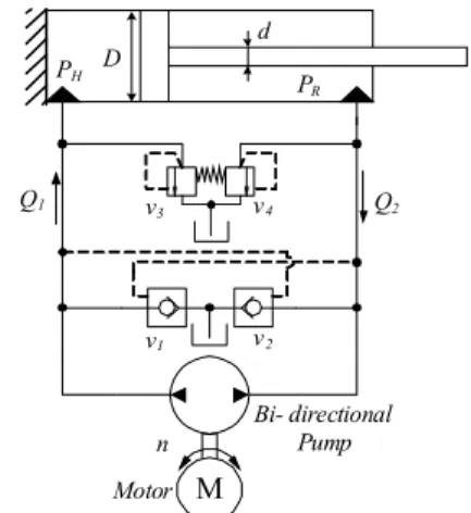
at Moog, Inc. (East Aurora, NY).Schematic of the

EHA is shown in figure 1. Here, the position of

hydraulic cylinder is adjusted directly by the

operation of the bi – directional pump. Obviously, the EHA acts as a Power –Shift which shifts the power from high-speed electric motor to the high-force of hydraulic cylinder. Thus, the EHA creates a sleeker, cleaner way to produce hydraulic power with higher energy efficiency, as proven by Rahmfeld and Ivantysynova ⁴⁾ . Because of its advantage, the EHA has been developed as commercial produces, e.g., the mini motion package from Kayaba Industry Co. ⁵⁾ , or the intelligent hydraulic servo drive pack from Yuken Kogyo Co. ⁶⁾ .

Contrary to the advantages of simple structure and good efficiency, the control of EHA is very complicated due to the nonlinearity and the large uncertainties of hydraulic systems. The nonlinearities originate from dynamics of piston pump and the actuating cylinder while the uncertainties is due to the unstableness of hydraulic parameters such as bulk modulus, compressibility and viscosity of oil, etc. Since the EHA possesses dead – zone when the pump changes direction, the control problem of EHA becomes even more challenging.

In literatures, the control of hydraulic valve - cylinder system has been studied for years. To deal with nonlinearity and uncertainty problems, the adaptive sliding mode ⁷⁾ , and the adaptive backstepping ⁸⁾ algorithms have been adopted.

However, the use of these techniques for the position control of EHA is surprisingly rare.

The position control of EHA has been introduced by Ahn et al. ⁹⁾ using Quantitative Feedback Theory (QFT). The controller design starts with experimental analysis on frequency response of EHA. Then, the controller is calculated for EHA to satisfy the control criteria for step response. Although the QFT control provides sufficient results in position control of EHA, the development of other control technique for EHA is an interesting topic.

This paper presents a position control of an EHA system using adaptive sliding mode

technique. Firstly, the dynamic model of EHA is investigated. Then, the position control using backstepping technique with adaptive rules is developed. The control signal consists of an adaptive control signal to compensate nonlinearities and a simple robust structure to deal with the bounded disturbance. Finally, experimental results are carried out to evaluate the effectiveness of the proposed control method.

The remainder of this paper is organized as follows. In Section 2, the mathematical model of the EHA is described. Then, the position controller is designed in Section 3, while experimental results are carried out in Section 4. Finally, Section 5 gives some conclusions.

M

P

H

P

R

Q

1

Q

2

D d

n v

1

v

2

Motor

Bi- directional Pump v

4

v

3

Fig. 1 Electro–Hydrostatic Actuator

2. Modeling of EHA system

2.1. Experimental apparatus

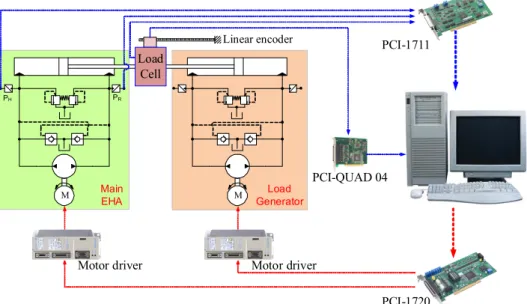
Schematic diagram of the whole system which

is consideration subject in this work is shown as

Fig. 2. The system consists of a PC based control

system, sensing system, and two electro –

hydrostatic actuators (EHA), which serve as

motion generator (main EHA) and load simulator

(load generator). In this configuration, the

movement of main cylinder is adjusted by the

speed of an AC servo motor (SGDM-50ADA)

through a fixed displacement piston pump,

reservoir and hydraulic control circuit. One linear

encoder, two pressure transducers and one load

M

P

H

P

R

M

Motor driver

Linear encoder

Motor driver

PCI-1711

PCI-1720 PCI-QUAD 04 Load

Cell

Main

EHA Load

Generator

Fig. 2 System schematic Diagram

cell are installed to the system to measure the cylinder position, the pressure of two chambers of the main EHA and the loading force, respectively.

One encoder, Quad – 04 card by Measure Computing Corp., and two multi-function data acquisition cards, A/D 1711 and D/A 1720 by Advantech, are installed on the PCI slots of the PC to perform the peripheral interfaces. In order to evaluate the main EHA system for variant working conditions, the load simulator is installed.

Generated load to the main cylinder is adjusted via force control applied to the load generator.

For the position control task, the processing system is built on a personal computer (Intel ® CoreTM2 Duo 1.8 GHz) within Simulink environment combined with Real-time Windows Target Toolbox of MATLAB. This processing system calculates the control signal based on the feedback states e.g., cylinder position, pressure of two chambers of main EHA, and loading force on main cylinder to adjust the position of the main cylinder. Control signal is in the form of analog voltage signal which is sent to the main EHA driver from PC through the 1720 D/A converter.

Meanwhile, the position information from the linear encoder is captured through interface of the PCI Quad – 04. Other data from load cell and two pressure transducers are sent back to the PC

through the 1711 A/D converter. Setting parameters for the EHA system are shown in Table 1.

2.2. Mathematical model

Consider EHA system (as shown in Fig. 3), the dynamics of the piston can be described by:

H H R R

my P A && = − P A − F (1) where,    is the equivalent mass, stiffness and damping, respectively;  is system displacement;  _   _ are pressure in two chambers respectively;  _   _ are actuating areas respectively; and  is external loading force.

Assuming there is no external leakage, the dynamics of cylinder oil flow can be written as:

( )

( )

( )

( )

01

02

H e H H t H R

H e

R R R t H R

R

P Q A y C P P

V A y

P Q A y C P P

V A y β

β

⎧ = − − −

⎪ +

⎪ ⎨

⎪ = + + −

⎪ −

⎩

& &

& & ₍₂₎

Where:   is the coefficient of the internal leakage

of the cylinder,  _ is the effective bulk modulus of

the hydraulic fluid in the container,     _ are

the original total control volumes of the two

chambers respectively (including the volume of

pipelines and initial cylinder chambers),  _

represents the supply flow rate to the H chamber (or cylinder end), and  _ represents the supply flow rate to the R chamber (or rod-end).

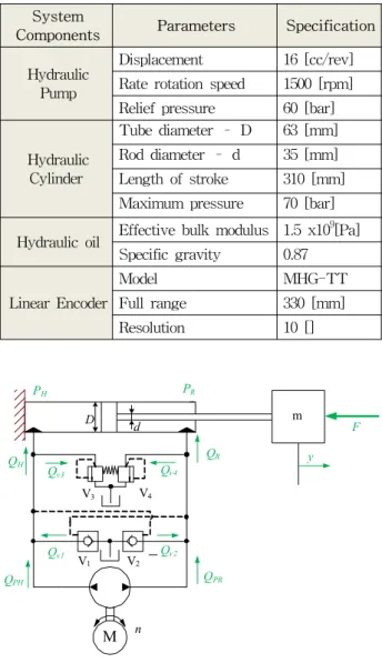
Table 1: Setting parameters for EHA system.

System

Components Parameters Specification

Hydraulic Pump

Displacement 16 [cc/rev]

Rate rotation speed 1500 [rpm]

Relief pressure 60 [bar]

Hydraulic Cylinder

Tube diameter – D 63 [mm]

Rod diameter – d 35 [mm]

Length of stroke 310 [mm]

Maximum pressure 70 [bar]

Hydraulic oil Effective bulk modulus 1.5 x10

⁹

[Pa]

Specific gravity 0.87

Linear Encoder

Model MHG-TT

Full range 330 [mm]

Resolution 10 []

M

P H P R

Q H Q R

D d

m

n

y

V

3

Q v1 Q v2

Q v3 Q v4

Q PH Q PR

F

V

4

V

1

V

2

Fig. 3 EHA system with load

Flow rates into two chambers are calculated as:

1 3

2 4

H PH v v

R PR v v

Q Q Q Q

Q Q Q Q

= + −

⎧ ⎨

= + −

⎩ ⁽³⁾

where Q ^PH = − Q ^PR = Q ^pump is the supplying flow rate from the pump:

( )

pump leakage H R

Q = D ω − k P − P (4)

where,  _{} is the leakage constant,  is displacement of the pump, and  is the input

driven speed from the servo system.

2.3 Control problem statement

In normal operation, the system pressure values:

 _   _ should be kept under the setting value

 _ of two relief valves V 3 and V 4 . It means that the flowrates through the two relief valves  _ ,

 _ are zero. Consequently, equation (3) can be rewritten as:

1 2

H PH v

R PR v

Q Q Q

Q Q Q

= +

⎧ ⎨

= +

⎩ ⁽⁵⁾

Define the state vector as

( ^{1 , , , , 2 3 4} ) ( ^{T , , H , , R} ) ^T

x = x x x x ≡ y y P P & ,

The simplified mathematical model of EHA system can be described by employing (1-4):

( )

1 2

2 3 4

1

H R

x x

x A x A x F

m m

=

= − −

&

&

( ) ^{( )}

)

( ) ^{( )}

)

3 3 4

01 1

1 2

4 4 3

02 1

2 2

e

leakage t H

v H

e

leakage t R

v R

x D k C x x

V A x Q A x

x D k C x x

V A x Q A x

β ω

β ω

= + ⎛ ⎜ ⎝ − + − +

− −

= ⎛ ⎜ − − + − +

− ⎝

− +

&

&

(6)

Let

3 4

34 A x H A x R

x m

= − _, ^{d F}

= − m , k ^leak = k ^leakage + C ^t ,

1 A H e

m β = β , ²

A R e

m β = β

, and

2

eq d

k C

= ρ

, the state space can be rewritten in strictly feedback form as:

( )

( )

( )

( )

1 2

2 34

1 2

34

01 1 02 1

1

1 3 4

01 1

2 2 3 4 2

01 1

2

H R

v leak H

H

v leak R

R

x x

x x d

x D

V A x V A x

Q k x x A x

V A x

Q k x x A x

V A x

β β ω

β

β

=

= +

⎛ ⎞

= ⎜ + ⎟ +

+ +

⎝ ⎠

+ ⎛ ⎜ ⎝ + − − − − +

− − + − + ⎞ ⎟

− ⎠

&

&

&

(7)

Obviously, the system states are adjusted by the

speed of the bi –directional pump which is driven by an AC servo motor. Given a bounded desired trajectory  _ , the objective of this paper is to determine the input speed command for the AC servo motor  to control the output position  _ track as closed as possible to  _ .

3. Control design

In this section, the position control is developed basedon adaptive backstepping technique. The backstepping controller is constructed to find out the input speed command  as follows.

Step 1. Define the tracking error as:

1 1 d 1

z = − x x

The derivative of tracking error is as follows:

1 2 d 1

z & = − & x x ₍₈₎

Let

2 1 1 1 1

2 2 2

, 1

d d

d

x x k z k

z x x

= − >

⎧ ⎨

⎩ = −

&

It follows that

2 1 1 1

z = + z & k z ₍₉₎

Here, if  _ →, then  _ →. Thus, the next step is to control   as small as possible.

Step 2. Note that

2 2

d

2 34 1

d

1 1

z & = − x & x & = x + − d x && + k z &

Let

34 1 1 1 2 2 2

34 34 34

, 1

d d

d

x x k z k z k D

z x x d δ

+

⎧ = − − =

⎪ ⎨

⎪ = − +

⎩

&& &

where,   sup, and  is the acceptable boundary of error  _ .

Then

34 2 2 2

z = z & + k z + d ₍₁₀₎

Obviously, if we can control the error  _ at small value, then the error   is bounded around

. Hence, next step is to control the error  as

small as possible.

Step 3. This step aims to synthesize an actual control law for the input  of the system. Rewrite the last equation of (7) as

( ) ( )

1 ( ) 2

34

h x h x

x g x

ω +

=

&

(11) where

( ) ( )( )

( )

01 1 02 1

2

01 02 02 01 1 1

0

H R

H R H R

g x V A x V A x

V V V A V A x A A x

= + −

= + − − ≥

( ) ( )

1 02 A 01

h x = β V + k V β D

( ) ( ) ( ( ) )

( ) ( ( ) )

( )( )

( ) ( )

( ) ( )

( ) ( )

2 02 1 1 3 4

01 1 2 3 4 2

01 02 3 4

01 02 2 1 2 1

1 3 4

1 2 1 02 2 01

R v leak H

2

A A H v leak R

leak A leak

R A H v R v A H

leak R leak A H

R H A H R v v A

h x V A x Q k x x A x

k V k A x Q k x x A x k k V k V x x

A k V A V x Q A Q k A x k A k k A x x x

A A k A A x x Q V Q k V k

β β

β β

β β

β β β β

β β

β β β β

= − − − − −

− + − + − +

= − + −

− + + +

+ − −

+ − + − +

= −

( )( )

( ) ( )

( ) ( )

01 02 3 4

01 02 2 1 2 1

1 2 1 02 2 01

leak A leak

R A H v R v A H

R H A H R v v A

k V k V x x

A k V A V x Q A Q k A x A A k A A x x Q V Q k V

β β

β β β β

β β β β

+ −

− + + +

+ − + − +

Define the uncertain parameters set

[ ^{1 2 3 4 5 6 7 8} ] ^T

α = α α α α α α α α

as

1 V V 01 02

α = _,

2 V A 02 H V A 01 R

α = − _,

3 V 02 k V A 01

α = β + β _,

4 k k V leak A 01 k leak V 02

α = β + β _,

5 A k V R A 01 A V H 02

α = β + β _,

6 Q v 1 A R Q k v 2 A A H

α = β + β _,

7 A A R H k A A A H R

α = β − β _,

8 Q k V v 2 A 01 Q v 1 V 02

α = β − β

Then,

( ) ^{1 2 1 H R 1 2 0}

g x = + α α x − A A x ≥ ( )

1 3

h x = α D

( ) ( )

2 4 3 4 5 2

6 1 7 1 2 8

h x x x x

x x x

α α

α α α

= − − −

+ + +

Since   ≥ , define the Lyapunov function as

2 34

1 ( )

V

=2

g x z (12)

The derivative of (12) is calculated as follows

( )

( )

2

34 34 34

2 2

2 2 34 1 2 34 34 3

34 4 3 4 5 2

6 1 7 1 2 8

2

34 1 2 1 1 34

1 ( ) ( )

2 1

2 ^{H R}

H R d

V g x z g x z z

x z A A x x z z D

z x x x

x x x

z x A A x x

α α ω

α α

α α α

α α

= +

= − +

+ ⎛ ⎜ − − −

⎝

+ + + ⎟ ⎞

⎠

− + −

& & &

&

(13)

Here, the derivative of x& ^34d is calculated as

( )

34 d 1 d 1 1 2 2 1 d 1 1 2 1 1 1

x & = &&& x − k z && − k z & = &&& x − k z && − k z && + k z &

Let α ˆ _i is the estimated value of α _i , i ⁼ 1, 2,...,8 _,

we design the control input law as follows.

( ^{ω ω ω ˆ 1 3 ˆ x D 2 4 1} ) ³

ω α α

+ +

= + (14)

( )

( )

(

1 1 2 34 1 34

2 2 2 34

5 6 3 4 7 2

1 ˆ 2

ˆ ˆ ˆ

H R d

A A x x z x x x z

x x x

ω

ω α

α α α

= −

= −

− + − + +

&

( ) )

( )

8 1 9 1 3 4 10 1 2

1 2 1 34

ˆ ˆ ˆ

ˆ ˆ _d

x x x x x x

x x

α α α

α α

+ + − +

+ + &

( )

3 k z 3 34 k Dsign z 4 34

ω = − −

where,   is used to compensate the certain known factors,   is the adaptive signal, which is employed to deal with uncertainties, and   is the robust signal which deals the disturbance .

For simplicity, define

[ ]

[ ]

[ ]

1 2

1 3 4

2 5 6 7 8 9 10

T g

T h

T h

α α α

α α α

α α α α α α α

=

=

=

The estimation of uncertain parameters α ˆ _{g ,} α ˆ _h 1

and α ˆ _h ² can be done as follows. Consider the Lyapunov function:

( ^{1 1 1 1 1 2 2 1 2} )

1 2

T T T

a g g g h h h h h h

V = + V α T ⁻ α α + T ⁻ α + α T ⁻ α

where, T T _g , _h ¹ , and T are the positive definite _h ² constant diagonal matrixes. In order to ensure

a 0

V & ≤ , the update law is chosen as follows:

( )

( )

1

34 34 34

1 1 34 1

2 2 34 2

ˆ 1 2

2 ˆ ˆ

h

g g d

h h

h h

T z gz gx proj T z h T z h

α

α

α ω

α

= −

=

=

& & &

&

& ⁽¹⁵⁾

where,

( ) ( )

( )

1 1 1

2 2 2

T g T h T h

g g x h h x

h h x α

α α

=

=

= and

( )

1

1 1max

1 1min

0, ˆ * 0

* 0, ˆ * 0

*,

h

h h

h h

if and

proj if and

otherwise

α

α α

α α

= >

⎧ ⎪

= ⎨ = <

⎪ ⎩

4. Experimental results

In this section, experiments for the system using the designed backstepping controller as described in section 3, are carried out. The controller is tested with two conditions: a unloaded motion and a bounded 16KN loaded motion. A sinusoidal signal is employed as reference position control.

 _ =100sin(0.1pt) [mm]

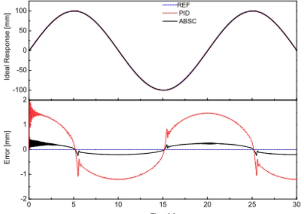
The control results are shown in fig. 4 and fig.

5. For unloaded condition, the effect of dead – zone, while the pump changes direction, is shown clearly. When the pump changes its movement direction, there is always a peak error as seen at time 5.1s, 15.1s, and 25.1s on the error graph. As seen in fig.4, the developed backstepping control provides better response than the PID controller.

The proposed backstepping control with adaptive laws also reduces the dead –zone effect on the system response. However, the chattering phenomena still occurs in the system response.

In the 16KN loaded condition, while the PID

cannot maintain good response, the proposed controller still provides acceptable response. These experimental results prove that the designed controller have strong ability to be applied as the position control for a nonlinear system as the EHA.

5. Conclusions

A modified backstepping position control has been presented for a nonlinear EHA with uncertainties. The control structure is designed by selecting a special Lyapunov function, while all uncertain terms are adapted by selecting another Lyapunov function. The whole control structure is the combination of adaptive technique and a simple robust structure to compensate the nonlinearities and bounded disturbance. Experimental results prove that the proposed controller can obtain accurate performance even in the presence of an external disturbance.

0 5 10 15 20 25 30

-2 -1 0 1 2

Er ro r [m m]

Time [s]

-100 -50 0 50

100

^REF _PID

ABSC

Ideal R e spons e [ m m ]

Fig. 4 Sinusoidal response in no loaded condition

-100 -50 0 50

100

Ref

PID ABSC

Error [mm]

Time [s]

Loaded Response [mm]

0 10 20 30

-4 -2 0 2 4

Fig. 5 Sinusoidal response in 16kN loaded condition

Acknowledgements

This research was supported by the research fund of the Mechanical Engineering, University of Ulsan, Korea.

References

1) J. I. Yoon et al., “Development of Hybrid Excavator for Regeneration of Boom Potential Energy”, Trans. of KFPS, Vol. 6, No. 4, pp.

1-8, 2009.

2) S.W. Choi and J. Y. Hur, “Dynamic Analysis on the Tail Gate System for Vehicle with the Energy Regenerative Brake of Hydraulic Driven Systems”, Trans. of KFPS, Vol. 7, No.

2, pp. 19～26, 2010.

3) S. H. Cho, “Path Control with Energy- Saving Load-Sensing for a Cylinder-Load System Using Speed-Controlled Fixed Displacement Pump,” Trans. of KFPS, Vol. 6, No. 3, pp. 1 6～22, 2009.

4) Rahmfeld, R., & Ivantysynova, M.,

"Displacement controlled linear actuator with differential cylinder—A way to save primary energy in mobile machines", Proc. of the 5th Int. Conf. on Fluid Power Transmission and Control, Hangzhou, China, pp. 316–322, 2001.

5) Kayaba Industry Co., Ltd., Mini-Motion Package Catalog.

6) Yuken Kogyo Co. Ltd., Intelligent Hydraulic Servo Drive Pack Catalog.

7) Guan C, Pan S., "Adaptive sliding mode control of electro-hydraulic system with nonlinear unknown parameters", Cont. Eng.

Prac., Vol. 16, No. 11, pp. 1275-84, 2008.

8) Ursu I, Ursu F, Popescu F., "Backstepping design for controlling electrohydraulic servos",Journal of the Franklin Institute Vol.

343, No. 1, pp. 94-110, 2006.

9) K.K. Ahn, N.H.T. Chau, D.Q. Truong,"Robust force control of a hybrid actuator using quantitative feedback theory", Journal of Mechanical Science and Technology, Vol. 21, No. 12, pp. 2048–2058, 2007.

10) H. E. Merritt, Hydraulic Control Systems. New York: Wiley, 1967.

11) N.D. Manring, Hydraulic Control Systems,

Wiley, 2005.