Simulation of Mobile Robot Navigation
based on Multi-Sensor Data Fusion by Probabilistic Model
Tae–seok Jin1*
<Abstract>
Presently, the exploration of an unknown environment is an important task for the development of mobile robots and mobile robots are navigated by means of a number of methods, using navigating systems such as the sonar-sensing system or the visual-sensing system. To fully utilize the strengths of both the sonar and visual sensing systems,
In mobile robotics, multi-sensor data fusion(MSDF) became useful method for navigation and collision avoiding. Moreover, their applicability for map building and navigation has exploited in recent years. In this paper, as the preliminary step for developing a multi-purpose autonomous carrier mobile robot to transport trolleys or heavy goods and serve as robotic nursing assistant in hospital wards. The aim of this paper is to present the use of multi-sensor data fusion such as ultrasonic sensor, IR sensor for mobile robot to navigate, and presents an experimental mobile robot designed to operate autonomously within indoor environments. Simulation results with a mobile robot will demonstrate the effectiveness of the discussed methods.
Keywords : Navigation, Sonar sensing, Mobile Robot, Control model
1* Corresponding Author, Professor Dept. of Mechatronics Dept. of Smart Electronics Control (E-mail: [email protected])
1. Introduction
A mobile robot has many application fields because of its high workability. Especially, it is definitely necessary for the tasks that are difficult and dangerous for men to perform.
There are many people who are interested in the mobile robot. However, most of them are aiming at successful navigation, that is, focusing on recognizing a location and reaching at a fixed destination safely.
Probabilistic methods have been shown to be well suited for dealing with the uncertainties involved in this problem. The method is based on a variant of the EM (expectation–maximization) algorithm, which is an efficient hill-climbing method for maximum likelihood estimation in high- dimensional spaces. In the context of mapping, EM iterates two alternating steps: a localization step, in which the robot is localized using a previously computed map, and a mapping step, which computes the most likely map based on the previous pose estimates [1][2].
This paper also implements sonar sensor- based on-line map building that is based on the application of the Hough Transform [3].
This approach builds a map of straight line geometric primitives which is then combined with the sensor fusion approach using local map data, resulting in an improved new method, allowing the system to make a more efficient use of collected sensory information for simultaneous and cooperative construction
of a world model and learning to navigate to the goal.
2. Implementations 2.1 Sonar Scanning
Sonar has unique properties which make it very useful for mobile robot navigation. The transducers are cheap, reliable, and physically robust, and they can ‘see’ a wide variety of objects since most solids are good sonar reflectors. Most significantly, accurate, robust range estimates are easy to extract from sonar data. These can be used for obstacle avoidance and are often difficult to obtain by other means.
These features combine to make the interpretation of sonar readings very difficult, while the low speed of sound forces sampling rates to be kept quite low (10-20 Hz for ranges up to 10 meters) and puts a premium on effective data interpretation [4].
A high-resolution sonar scan of an empty room is shown in fig. 2 (from [5]). This was taken by firing a rotating Polaroid sensor at 5 degree intervals and plotting apparent range against sensor-axis angle, as shown in Fig. 3
2.2 Object Classification
For many years, a lot of work has been invested in generating maps for mobile robots by ultrasonic sensors with or without
classification of environment objects as shown in Figure 2.
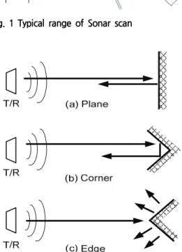
Fig. 1 Typical range of Sonar scan
Fig. 2 Reflection behavior of a) planes, b) corners, and c) edges
The main goal is still to find collision free paths for a given destination in an unknown environment. Generally, successful path planning strategies require sufficiently accurate information about the mobile robot’s position.
This is usually not satisfied by pure odometric measurement because of the accumulation of errors in the progress of robot’s motion [9].
Therefore, pose tracking requires frequently recalibration. Additional information about the surroundings of the robot from sensor devices or offline prepared maps is needed. In the case of sensory generated maps, it is a question of precision and reduction of ambiguities to include information about echo causes and object shapes, respectively. In recent years, mainly two ways became apparent for map building and object classification purposes:
1) based on sensor arrays, capable of gathering information without sensor movement [6] ;
2) based on a few sensors utilizing typical scanning movements (e.g., rotary scans) [7], [8].
Because of unknown echo direction inside the sound lobe, the sensor axis is often used as representation of the echo direction for each measurement. Rotary scans on different positions using this simple geometric interpretation leads to the typical regions of constant depth (RCDs) which can be used to build a map [2]. The different reflection behavior of different object types (Fig. 2) influences the length of RCDs. In combination with amplitude information, this can be used to distinguish planes, edges, and corners [9],[10].
2.3 Feature Extraction with Hough Transform
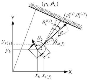
With the sonar model presented as Fig. 3, associating sonar returns to line segment geometric primitives may be stated as finding groups of sonar arcs all tangent to the same line.
Given the large amount of spurious data coming from moving people, specular reflections and sonar artifacts, the Hough Transform [7] seem very appropriate for the following reasons: 1) The location of line features can be easily described with two parameters, giving a 2D Hough space in which the voting process and the search for maxima can be done quite efficiently; 2) The sonar model presented can be used to restrict the votes generated by each sonar return to be located along the corresponding transformed sonar arc; 3) Since each sonar return emits a constant number of votes, the whole Hough process is linear with the number of returns processed; and 4) Being a voting scheme, it is intrinsically very robust against the presence of many spurious sonar returns.
If the location of the robot at time is known, which can be obtained through the accumulation of encoder information. For more accuracy of the algorithm, we should consider the mounted position of each sonar sensor.
) , (pk k
) , (pks(j) ks(j)
) ( j ks
) ( j
s
kL
xk xs( j)
y
k) ( j
y
sFig. 3 Modeling of Sonar Ring
The value of each sonar sensor offsets robot heading is ( ⋯), is the sequence number of sonar, and Pioneer-DX mobile robot has 16 sonar sensors in all), which is invariable. Consequently, the
sonar sensor position () in the state space is given in(1)∼(4):
⋯ (1)
⋯ (2)
cos (3)
sin (4)
Where is the eccentric distance of sonar sensor, the value of can be given in (6), which is the position of the extracted line segment represented in a base reference for:
(5)
cos sin (6)
One of the key issues of its practical implementation is choosing the parameters defining the Hough space and their quantization. In our implementation, we perform some prior filtering for removing noisy data. Two filtering operations on sonar data points are used. First the sonar returns obtained along short trajectories(2m), which above a certain limit, distance readings were not very reliable, and thus were rejected. A second filtering operation, Let be a set of sonar data points. A point is rejected, if no other data point of is found inside a circle of radius and center at .
Excellent results have been obtained with data sets , which coming from a number of consecutive sonar-rings cans. In order to keep the odometry errors small,lines are represented in a base reference, using parameters and
defining the line orientation and its distance to the origin (Fig. 3).
3. Data Fusion by Probabilistic Model
Data fusion is about deriving information about certain variables from observations of other variables. The application area is huge, see the special issue on data fusion in [3] for a recent overview. An edited collection of survey papers on data fusion in robotics and machine intelligent is given in [6]. Sensor
fusion in general is discussed in [7].
From a probabilistic perspective, we have the following problem. Given two vector random variables and , what does the observation tell us about ? The complete answer is given by the so-called conditional probability density function,
(7)
Here is the joint probability density for and , and is the probability density for . By using the dual as sumption, namely that is given, we obtained the very useful Bayes rule
(8)
(9)
which is the key formula in Bayesian and maximum likelihood estimation theory.
Different estimates of can now be constructed from its distribution. The (conditional) minimal variance of equals the conditional mean of given ,
∞
∞
(10)
Another useful estimate is the maximum a posteriori estimate, which maximizes the function . The rest is design and
analysis issues, i.e. formulating the underlying model, specifying probability density functions and calculating equality/variance properties.
The most used probability density function is the Gaussian one(the Normal distribution).
The main reason is that the conditional density function also will be Gaussian, and analytic expressions of the minimal variance estimate can thus be obtained.
Let and be jointly Gaussian, i.e.
′′ is Gaussian with mean and covariance
∑
∑∑
∑∑
(11)
Then conditional on has a Gaussian distribution with mean and covariance,
∑∑
∑ ∑ ∑∑ ∑
(12)
Hence the conditional mean of given
, equals
∑∑ (13)
Almost all practical estimators are special cases of the above result. The expression is called the fundamental equations of linear estimation in [10]. This reference also provides a very good introduction to estimation theory, in general, and tracking, in particular.
4. Simulation Setup and Results
We setup a mobile robot for simulation, and use an ultrasonic sensors are used for the navigation control. The ultrasonic sensor is used for recognizing environment, which is rotated by a step motor within 180 degrees;
the CCD camera is used for detecting obstacles.
Single Sensor Data Fusion(SSDF)and Multi- Sensor Data Fusion(MSDF)have first been tested with experimentation to show the usefulness of MSDF in two environments respectively. Starting at (0.3m, 5m, 0 degree), avirtual robot was driven around a virtual square corridor onetime.
In each round, the mobile robot stops a total of 12times to rescan the environment.
The size of given map is 12m X 8m, the total distance traveled is 12 + 8=20meters, and the total number of scanning points is 38. The comparison of navigation trajectory at all stops is shown in Fig. 4 and Fig. 5.
Figure 4 shows determination of the pointing vector based upon only current readings used SSDF. This robot was made to move randomly within the confines of the above setup and at the region, . There are a little of difference between SSDF and MSDF.
But at the rest of region, the robot moves keeping the distance between robot and obstacles constant and have some difficult local minimum trap problems at some places.
Fig. 4 Experimental result used a SSDF scheme
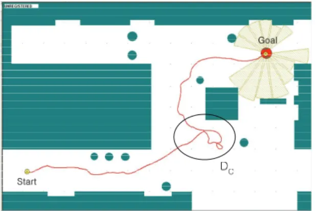
Figure 5 shows MSDF scheme is applied for the measurement. And the results are compared to show the superiority of the proposed scheme. The robot was allowed to move keeping the distance between robot and obstacles constant at the region, .
The region , shows the improvement in steering at boxes obstacle. And the navigation experiments show that a mobile robot, utilizing MSDF scheme, can avoid obstacles and reach a given goal position in the workspace of a wide range of geometrical complexity. Experiments results using MSDF, show the robot can avoid obstacles (boxes and trash can) and follow the wall.
Figure 4 and Figure 5 demonstrate one of many successful experiments. The algorithm is very effective in escaping local minima encountered in laboratory environments.
The mobile robot navigates along a corridor with 3m width and with some obstacles as shown in Figure 5. It demonstrates that the mobile robot avoids the obstacles intelligently and follows the corridor to the goal.
Fig. 5 Experimental result used a MSDF scheme
5. Conclusion
In this paper, we have described progress towards a vehicle localization system based on detailed physical and probabilistic modelling of the sonar sensing process, which promises to provide one substantial piece of this capability.
From a scientific/academic perspective it is important to study very general issues and approaches, were the ultimate aim is full autonomy. However, the engineering perspective is the opposite, i.e. one wants to solve a specific problem, e.g. a sonar sensor based feedback control algorithm for going through narrow doorways. However, the main issue for such research is scalability, i.e. is the solution of more general interest and can it be extended to more complex situations.
References
[1] J. Leonard, H. Durrant-Whyte, “Mobile robot localization by tracking geometric beacons”, IEEE Transactions on Robotics and Automation, vol.7, no.3, pp. 376-382, (1991).
[2] H.-J. Von der Hardt, D. Wolf, R. Husson, “The dead reckoning localization system of the wheeled mobile robot ROMANE”, Multisensor Fusion and Integration for Intelligent Systems 1996. IEEE/SICE/RSJ International Conference on, pp. 603-610, (1996).
[3] J. Borenstein, H. Everett, L. Feng, D. Wehe,
“Mobile robot positioning: Sensors and techniques”, J. Robotic Syst., vol.14, no.4, pp.
231-249, (1997).
[4] Le-Jie Zhang, Zeng-Guang Hou, Min Tan,
“Kalman filter and vision localization based potential field method for autonomous mobile robots”, Mechatronics and Automation 2005 IEEE International Conference, vol. 3, pp.
1157-1162, (2005).
[5] Chen Ling, Hu Huosheng, K. McDonald-Maier,
“EKF Based Mobile Robot Localization”, Emerging Security Technologies (EST) 2012 Third International Conference on, pp. 149-154, 5-7 Sept. (2012).
[6] C Suliman, F Moldoveanu, “Unscented Kalman lter position estimation for an autonomous mobile robot” in, Bulletin of the Transilvania University of Brasov, Series I: Engineering Sciences, vol. 3, no. 52, (2010).
[7] Q. Meng, Y. Sun, Z. Cao, “Adaptive extended Kalman filter (AEKF)-based mobile robot localization using sonar”, Robotica, vol. 18, no.
5, pp. 459-473, (2000).
[8] V. Malyavej, W. Kumkeaw, M. Aorpimai,
“Indoor robot localization by RSSI/IMU sensor fusion”, Electrical Engineering/Electronics Computer Telecommunications and Information Technology (ECTICON) 2013 10th International Conference on, pp. 1-6, (2013).
[9] E. North, J. Georgy, M. Tarbouchi, U. Iqbal, A.
Noureldin, “Enhanced mobile robot outdoor localization using INS/GPS integration”, Computer Engineering & Systems 2009. ICCES 2009. International Conference on, pp. 127-132, (2009).
[10] D.M.G.A.I. Sumanarathna, I.A.S.R. Senevirathna, K.L.U. Sirisena, H.G.N. Sandamali, M.B. Pillai, A.M.H.S. Abeykoon, “Simulation of mobile robot navigation with sensor fusion on an uneven path”, Circuit Power and Computing Technologies (ICCPCT) 2014 International Conference on, pp. 388-393, (2014).
(Manuscript received May 6, 2018; revised June 21, 2018;
accepted July 9, 2018.)