Ionospheric Storm Detection Method Using Multiple GNSS Reference Stations

(1)

1. INTRODUCTION

In terms of GNSS augmentation systems, ionospheric storms began to draw attention after it was observed by WAAS reference stations (baseline length 40 ~ 100 km) distributed throughout the US at 20:15 UTC in November, 2003. The observed ionospheric storm had a slope of about 425 mm/km (Datta-Barua et al. 2008). Ionospheric storms are a threat to GNSS augmentation systems because it is difficult to predict when and where they will occur and how strong they will be. If the ground station of the augmentation system differs from the user’s ionosphere environment, errors occur in the correction information from the reference station, thus leading to increased user position errors (Hoffmann-Wellenhof et al. 2008). Therefore, based on previous cases, the US parameterized ionospheric storm

Ionospheric Storm Detection Method Using Multiple GNSS Reference Stations

Jongsun Ahn

¹

, Sangwoo Lee

¹

, Moonbeom Heo

¹

, Eunseong Son

¹

, Young Jae Lee

^2†

1

Korea Aerospace Research Institute, Daejeon 34133, Korea

2

Aerospace Information Engineering, Konkuk University, Seoul 05029, Korea

ABSTRACT

In this work, we propose detection method for ionosphere storm that occurs locally using widespread GNSS reference stations.

For ionosphere storm detection, we compare ionosphere condition with other reference stations and estimate direction of movement based on ionosphere time variation. The method use carrier phase measurement of dual frequency, for accuracy and precision of test statistics, are evaluated with multiple GNSS reference stations data.

Keywords: GNSS multiple reference stations, ionospheric storm detection, dual-frequency carrier phase

models for worst-case scenarios where ionospheric storms could affect GNSS local augmentation systems (Datta-Barua et al. 2010). We also estimated the maximum ionospheric storm slope observed in Korea based on data from multiple reference stations (2000 ~ 2004) distributed throughout the country (Kim et al. 2014).

Two types of methods have been proposed to detect ionospheric storms: a method that uses measurements that show different characteristics when GNSS system signals pass through the ionosphere, and a method that monitors the influence of the ionospheric storm on the user position error. In terms of measurements, the typical detection method is Code-Carrier Divergence (CCD).

The code and carrier measurements of the GNSS system are subject to different effects as they pass through the ionosphere, in which the code experiences a delay while the carrier experiences an advance. If the thickness of the ionosphere increases dramatically due to ionospheric storms, the difference between the two measurements gradually increases to the extent of divergence (Cho et. al 2015). Using this, the CCD method detects ionospheric storms based on the Geometric Moving Average filter with the time variation of the code and carrier difference values (Simili & Pervan 2006). However, as CCD is a detection method using code measurements, the precision of the test statistics may be low because of the noise included in Received Nov 13, 2018 Revised May 21, 2019 Accepted May 27, 2019

†

Corresponding Author

E-mail: [email protected]

Tel: +82-2-450-3358 Fax: +82-2-457-3358

Jongsun Ahn https://orcid.org/0000-0002-5432-4436

Sangwoo Lee https://orcid.org/0000-0002-0642-5064

Moonbeom Heo https://orcid.org/0000-0001-9674-9937

Eunseong Son https://orcid.org/0000-0002-0701-9965

Young Jae Lee https://orcid.org/0000-0002-9203-048X

(2)

in multiple reference stations are parallel, and thus has limitations in the detection range due to the limit of baseline length between multiple reference stations. In order to upgrade the accuracy and precision of test statistics and improve narrow detection range limits, this study proposed a method to compare the variation of ionospheric thickness of individual reference stations by using dual-frequency carrier and further estimate the direction of ionospheric storms.

2. MAIN TOPICS

2.1 Detection Method Configuration

First, calculate the variation of the ionospheric vertical delay over the individual reference stations based on the same satellites received from multiple reference stations through Dual Frequency Carrier Divergence (DFCD) based on dual-frequency carriers. Then, compare the variations among multiple reference stations and calculate the similarity of ionospheric storm thickness variation through the I-Value to detect ionospheric storms that occur over a specific reference station. Lastly, derive the inverse weights of the visible satellites based on the I-Value and estimate the direction of the ionospheric storm by applying the difference of DFCD between the reference stations to the least-squares method (Ahn 2015).

2.2 DFCD Inspection

DFCD refers to the time variation of geometry-free values of different frequency carrier measurements. This study developed an equation for geometry-free measurements based on the carrier measurement (Φ) of L1 and L2.

1 1

1 1 1 1 1 1

1 1 1

1 R c N 1 I f R f N f I

c c

δ δ

λ λ λ

Φ = + ∆ + − = + ∆ + − (1)

2 2

2 2 2 2 2 2

2 2 2

1 R c N 1 I f R f N f I

c c

δ δ

λ λ λ

Φ = + ∆ + − = + ∆ + − (2)

can be converted to geometry-free measurements that can offset the effect of the actual distance and the satellite clock error.

2 1

2 1 1

f

1 2 2 1 2

f

1

f f R f f f N f I

c δ c

Φ = + ∆ + − (3)

2 2

1 2 1

f

1 2 1 2 1

f

2

f f R f f f N f I

c δ c

Φ = + ∆ + − (4)

As shown in Eq. (5), if Eq. (3) is differenced by Eq. (4) and then divided by the L2 carrier frequency, only the effects of the integer ambiguity in each carrier and the ionospheric delay error will remain.

1 1 12

12 1 2 1 2 2

2 2 2 1

1 1 2

2 1

1 1 40.3 40.3

pp

f N f N f F VTEC

f f c f f

N f N b F VTEC

f f

 

Φ = Φ − Φ = − −  − 

 

= − − (5)

2 k

40.3

k

I = f VTEC , VTEC: Vertical Total Electron Content

2 12

1

^e

cos

ⁱ

pp e I

F R

R h θ

⁻

   

 

= −     +    

θ

ⁱ

: Elevation angle of satellite i at observing site (deg.) θ

^i'

: Zenith angles at the ionospheric point (deg.) h

_I

: 350 km (Mean value for the height of the ionosphere) R

e

: 6378.1363 km (Mean radius of the earth)

dt: Sample interval

In order to offset the effect of the integer ambiguity, time- differencing Eq. (5) and assuming that the variation of the obliquity factor over time is minimal will yield Eq. (6). At this point, we assume that the integer ambiguity of each carrier is the same. This allows us to monitor the variation of the ionosphere over time by excluding the constants included.

12

12 12 2

1 2

1 40.3

( ) t ( 1) t 1 f F t VTEC t

_pp

( ) ( )

f f c

 

Φ − Φ − = −  −  ∆

  (6)

Because the satellite elevation angle of the same satellite

is different for each reference station, the influence of the

(3)

ionosphere in the slant direction between the satellite and the reference station antenna may be different. In order to compare them from the same perspective, converting and organizing the slant direction values to vertical directions will yield Eq. (7).

12 12

1 12

( ) ( 1) 40.3

( )

_vert^DFC

pp

t t VTEC

DFCD t I

b f F dt f dt

Φ − Φ − ∆

= = − =

× × ×  (7)

12 22

1 1 f

b c f

 

=  − 

 

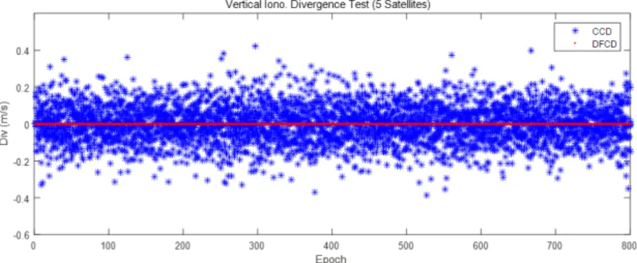
This paper defined Eq. (7) as the DFCD value and used it as a test statistic to monitor the time variation of the ionosphere thickness. To compare the degree of precision of the DFCD test statistic, we compared the CCD based on the code measurements with the same physical meaning and the test statistics under normal conditions, as shown in Figs. 1 and 2.

Fig. 2 is a histogram to derive the standard deviation of the test statistics, in which the X-axis represents the size of the test statistic and the Y-axis represents the number of samples. We can confirm the DFCD is a more precise test statistic value as the standard deviation (1 σ) of DFCD is 0.001 m/s compared to that of CCD (0.058 m/s). The precision of the test statistic can be configured as the precise threshold

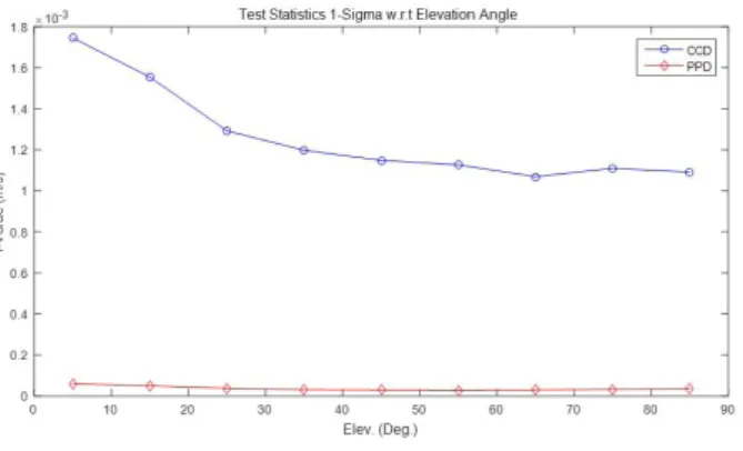
value to determine failure, thereby improving failure detection performance. Fig. 3 shows the ionospheric vertical delay according to the satellite elevation angle by using long-term data. It can be seen that there is a 5 to 25 times precision difference between DFCD and CCD.

Through statistically analyzing the test statistics according to the satellite elevation angle, the threshold value required for failure detection can be expressed as an exponential function as shown in Eq. (8) and Table 1.

Fig. 3. Ionospheric vertical divergence with respect to elevation angle.

Fig. 1. CCD and DFCD test statistics of normal condition.

Fig. 2. CCD and DFCD histogram of normal condition.

(4)

( ) e

⁽^b ⁾

e

⁽^d ⁾

i

a

^θ

c

^θ

σ θ =

⁺

+

⁺

, θ: Satellite elevation angle (in deg.) (8)

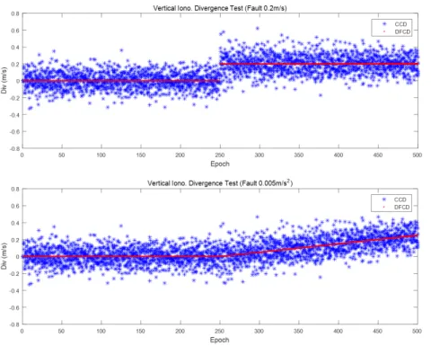
In addition, as a result of examining the accuracy of the test statistics in detecting the variation of ionospheric thickness by inserting a constant ionospheric vertical delay (0.2 m/s) and the vertical delay of a constant acceleration (0.005 m/s

²

) into the same satellites (5 satellites) as shown in Fig. 4, the DFCD value was found to be also superior to the CCD value in terms of accuracy.

2.3 I-Value Inspection

The satellites that have passed the DFCD inspection, which is an ionospheric vertical delay variation test, are checked for similarities with the DFCD values of the common satellites with neighboring reference stations.

This method is to monitor ionospheric storms with local error characteristics. If the I-Value of a specific satellite or a reference station in a specific region increases, we can suspect an ionospheric storm in that region. This can be expressed as Eq. (9).

1

1 1

1

m m

i i i

j n n

n n

n j

IV DFCD DFCD

M M

−

= =

≠

= −

∑ − ∑ ⁽⁹⁾

M: Number of multiple reference stations, j: Reference station index, i: Satellite index

The first term on the right side of Eq. (9) represents the mean DFCD value for the same satellite of M reference stations and the second term represents the mean DFCD value calculated for the rest of the reference stations except for the reference station in a specific region. By differencing this, we can calculate the I-Value of receiver j, which was excluded from the last term for satellite i. This is illustrated in Fig. 5. Assuming that the ionospheric storm is affecting satellite i received at reference station 1, the mean DFCD value of the entire reference stations for satellite I is increased by the DFCD value of reference station 1. At this point, in terms of differencing by the mean DFCD value of the reference stations other than reference station 1, they converge close to ‘0’ under normal conditions because the DFCD values are similar between the reference stations, but when an ionospheric storm occurs, the I-Value increases.

Fig. 4. Test result on simulated ionospheric storm condition.

Fig. 5. Conceptual diagram of ionospheric storm condition on multiple reference stations.

Table 1. Exponential function model of ionospheric delay variation (m/s).

Detection method a b c d

CCD

DFCD 0.004461

-0.000151 -0.07924

-0.07612 0.00411

0.00177 -0.00159 -0.02435

(5)

This indicates that the thickness of the ionosphere in the direction of satellite i is rapidly changing over reference station 1.

As in the case of DFCD, the standard deviation of the sample increases due to reduced noise as the elevation angle increases. Fig. 6 shows the results of analyzing this according to the satellite elevation angle.

As seen from the results in Fig. 6, it can be confirmed that the I-Value produced based on the DFCD value shows higher precision throughout the satellite elevation angle section compared to the I-Value based on CCD. Modeling this in the form of an exponential function is shown in Eq.

(10) and Table 2.

( ) e

⁽^b ⁾

e

⁽^d ⁾

iIV

a

^θ

c

^θ

σ θ =

⁺

+

⁺

, θ: satellite elevation angle (deg.) (10)

2.4 Estimating the Direction of the Ionospheric Storm Based on the De-weighted Least-squares Method

As the final step of detecting ionospheric storms, this study estimates the direction of the storm in relation to reference stations where the difference of DFCD values is relatively large through the I-Value. This allows the operator of the reference station to alert the areas that may be affected in advance based on the information of the ionospheric storm progressing in a particular direction.

Based on reference station A to detect the direction of the ionospheric storm, we can calculate the ionospheric delay relative to reference station B, as shown in Eq. (11). Project this into the location area to calculate the error due to the difference in the ionospheric delay error and estimate the direction of the ionospheric storm based on the direction of the error.

( )

i i i

AB B A

I DFCD DFCD t

∆ = − × ∆ (11)

Δt: Sampling time (sec)

The observation matrix to project into the location area is produced as shown in Eq. (12) by configuring a line-of-

sight vector based on the reference station coordinates, the satellite coordinates calculated from the satellite navigation messages, and the actual distance. The position

error is calculated by the least-squares method, as shown in Eq. (13). Eventually, the value derived from Eq. (13) is the error in Earth-centered Earth-fixed (ECEF) coordinate

system caused by the difference in the ionospheric delay error between two reference stations (A, B). By converting this into the Topocentric (ENU, East North Up) coordinate system, we can estimate the direction of the ionospheric

storm based on reference station (A).



1 1 1

1

2 2 2

1

A AB

A A A

i i i

A A A

AB A A A A

AB i i i

A

A A A

i A

AB i i i

A A A

i i i

A A A

x x y y z z

I x x y y z z x

I y

I z

x x y y z z

ρ ρ ρ

∆

 − − − − − − 

 

 ∆   − − −   ∆ 

 ∆   − − −   

  =    ∆  +

     ∆ 

 ∆     

 

    − − − − − −  

 

I x

H

 ε

  





(12)

( ) (

²

) (

²

)

²

i i i i

A

x x

A

y y

A

z z

A

ρ = − + − + − : Geometry truerange (m)

[ ]

ˆ

_A

x

_A

y

_A

z

_A ^T

∆ x = ∆ ∆ ∆ : Position error (ECEF, XYZ) x

A

, y

A

, z

A

,: Reference coordinate (ECEF, m)

( )

¹

ˆ

_A ^T ⁻ ^T _AB

∆ x = H H H I ∆ (13) 2.4.1 De-weighting-based least-squares method

In general, the measurements applied to the least- squares method do not all have the same error. Therefore, we use the weighted least-squares method as shown in Eq.

(14) by assigning different weights for each measurement and higher weights to satellites with relatively low errors.

( )

¹

ˆ

_u ^T ⁻ ^T

∆ = x H WH H W ρ ∆ (14)

1,2 1 2,2

,2

0 0

ⁱ

σ σ

σ

−

 

 

=  

 

 

W



   



(15)

However, in this study, we can increase the effect of estimating the direction by increasing the weights on the Fig. 6. I-Value variation with respect to elevation angle.

Table 2. Exponential function model of I-value (m/s).

Detection method a b C d

CCD DFCD

0.00059 -4.968e-005

-0.03464 -0.05884

0.001243 2.423e-005

-0.0041 0.001943

(6)

storms, instead of applying the reciprocal of the standard deviation of the measurement error as the weight.

1 2

0 0

d d d

id

w w

w

 

 

=  

 

 

W



   



(16)

,2, ,2

1

i i

d i iono n

w σ

= σ + (17)

σ

ⁱ

: Error standard deviation model under normal conditions (m) σ

ⁱiono

: Relative ionospheric vertical delay error standard deviation between network reference stations (m)

Eqs. (16) and (17) show the type of weights used in this paper, which basically reduce the weights due to error factors under normal conditions as in the case of conventional methods, but increase the weights of satellite measurements that are suspected of ionospheric storms.

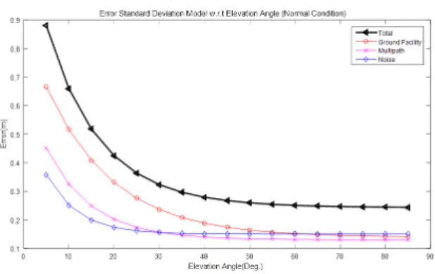
The error model under normal conditions and the related constants are shown in Eq. (18), and Tables 3 and 4 (U.S.

Federal Aviation Administration 2005). Based on Eq. (18), the size of the detailed factors constituting the error under normal conditions according to the elevation angle is as shown in Fig. 7.

,2 ,2 ,2

i i i i _

multipath noise pr gnd

σ = σ + σ + σ (18)

0.13 0.53

ⁱ10

multipathi

e

^θ

σ = +

⁻ ^

: Multi-path error model

0, 1, ,

i c AAD noisei

a

AAD

a

AAD

e

^θ^θ

σ = +

⁻

: User signal noise error model

(

^0, ^1, ^0,

)

²

₍ ₎

2

i _ 2,

i GAD

GAD GAD

pr gnd GAD

a a e

M a

θ θ

σ

+

−

= + : Reference station

error model

θ: Satellite elevation angle (Deg.), M: Ground reference stations (4 locations)

The de-weighted error model applies the standard deviation of the DFCD or CCD values generated by the

reference station. At this point, the standard deviation value after the normalization process is used as the sample to calculate the standard deviation.

,

i i

i CCD m

m n i

CCD

CCD µ CCD σ

= − (19)

_{m n}ⁱ_, ^DFCDⁱ _i ^mⁱ

DFCD

DFCD µ DFCD σ

= − (20)

The mean and standard deviation used in the normalization process were statistics under normal conditions; the mean was ‘0’ and the standard deviation was the model value based on Eq. (8) and Table 1. There is no problem in the normalization process under normal conditions, but in the event of an ionospheric storm, performing the normalization process with the values above is not appropriate from a statistical perspective. However, in terms of performing the normalization process with the values above from a failure detection perspective, we can easily derive values that are not normalized (mean ‘0’

standard deviation ‘1’). Calculating the standard deviation of the DFCD and CCD values of each reference station after performing normalization is as shown in Eq. (21).

( )

²

, 1

1

M i

i m m

iono DFCD

DFCD σ =

⁼

M

−

∑ , ( )

²

, 1

1

M i

i m m

iono CCD

CCD σ =

⁼

M

−

∑ (21)

2.4.2 Theoretical characteristics of the de-weighting-based least-squares method

This section will discuss the theoretical characteristics of the de-weighted least-squares method by numerically analyzing the unbiasedness and increase of variance. First, the configuration of the least-squares method to determine the theoretical Unbiasedness of the de-weighted least- squares method is as shown in Eqs. (22) and (23).

Fig. 7. Measurement error model of normal condition.

(7)

∆ = ∆ + I H X ε (22) ^ˆ (

^T d

)

¹ ^T d

∆ = X H W H H W I

−

∆ (23)

Substituting Eq. (23) into Eq. (22) leads to Eq. (24), and taking the expected value on both sides yields Eq. (25).

( ) ( )

( )

1 1

1

ˆ

^T _d ^T _d ^T _d ^T _d

I

T T

d d

− −

−

∆ = +

= ∆ +

X H W H H W H X H W H H W ε X H W H H W ε



(24)

( )

¹

_ [ ]

0

ˆ

^T ^T

E   ∆ X   = ∆ + X H WH H W ε

⁻

E (25)

The noise component ( ε) follows a Gaussian distribution, which results in the characteristics as shown in Eq. (26) if assuming that each error component is independent. By reflecting this, we can consider the expected value of the solution as estimated in Eq. (27) to be equal to the actual value. This shows that the least-squares method is unbiased even in the case of using the de-weighted weights.

0,

,2

i i i

E     ε = Var     ε = σ (26)

ˆ 0

E   ∆ X   − ∆ = X (27)

The estimation error variance of the conventional weighted least-squares method is as shown in Eq. (28), which helps to examine the characteristics of the variance.

( )

¹

ˆ

^T ^T

Var   ∆ X   = Var    H WH H W y

⁻

∆    (28)

Eq. (29) expresses this in the form of expected values.

[ ] ( ) [ ] ( )

( ) ( )

( ) ^ ( )

( )

1 1

1 1 1

1 1

1 T

T T T T

I

T T T

I T

E

⁻

E

⁻

− − −

− = −

−

∆ ∆ = ∆ ∆

=

W W

x x H W H H W y y W H H W H H W H H WW W H H W H

H W H H W H H W H H W H



  

(29)

If comparing the variances of the conventional weighted least-squares method and the de-weighted least-squares method using Cauchy-Schwarz inequality as shown in Eq.

(30), the size of the variance is determined according to the size of the weight.

T

≤

T

H W H H W H (30)

By comparing the size of the weights using Eq. (31), it can be seen that the variance of the de-weighted least-squares method is larger than that of the conventional weighted least-squares method, as shown in Eq. (32). Therefore, the de-weighted least-squares method is effective in terms of integrity rather than accuracy because it reacts sensitively to local ionospheric storms.



,2

,2 ,2

1 1

i i d

ionoi

i i

w w

σ _{} ⁺ σ ^≥ σ (31)

ˆˆ

_W _DW

Var   X   ≤ Var   X   (32)

Based on Eqs. (31) and (32), Fig. 8 shows how the weight

changes when there is a difference in the variation of

Fig. 8. Weighting variation of each satellites on ionospheric storm (PRN 16).

(8)

ionospheric vertical delay. In reality, changes in weight occur when there is a change in visible satellites over time;

thus, we assumed PRN 7, 16, 19, and 27 at any random time during the analysis period. If inserting a 0.001 m/s

²

failure in a specific reference station, PRN No. 16, after 12 o’clock, the weight would be calculated to be low by the conventional method because the elevation angle of satellite No. 16 is low, but the weight increases through the de-weighting process.

2.4.3 Ionospheric storm direction estimation simulation results

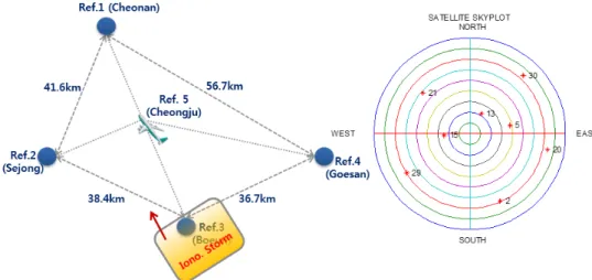
As shown in Fig. 9, this study used GNSS reference stations in 5 locations (Cheonan, Sejong, Boeun, Goesan, Cheongju) for simulation. The simulation was performed under the assumption that PRN No. 2 and PRN No. 20

received at Boeun reference station were influenced by an ionospheric storm (ionospheric vertical delay variation:

0.001 m/s2), individually or at the same time. The failure was selected to be of a size that can cause performance difference compared to CCD, which is currently used as the reference group. In addition, although the total data reception time was 24 hours as shown in Table 5, this study examined the results for 20 epoch (600 s) in order to review the changes in I-Values and weights in the same satellite group.

Under the assumption that the ionospheric storm may affect a single satellite or multiple adjacent satellites, we estimated the directions according to two scenarios. Fig. 10 shows the estimation results according to these scenarios.

As shown in Fig. 10, the CCD-based estimation method cannot estimate the direction of the ionospheric storm due to intrinsic noise. On the other hand, the DFCD method precisely maintains a position error close to ‘0’, and moves in the direction of PRN No. 2 at the moment a failure occurs, indicating an increase in error. Similarly, in the case of multiple satellites, the direction of the position solution Fig. 9. Simulation geometry condition of reference station and visible satellites.

Fig. 10. Estimation results of simulated ionospheric storm direction.

Table 5. Simulation data.

Receiver Date Time interval Total time

Trimble NETR5 or NetR9 2015. 04. 01 30 s 24 h

(9)

error indicates between PRN No. 2 and PRN No. 20.

3. CONCLUSTION

This paper proposed a method to detect ionospheric storms based on multiple reference stations. The detection method is divided into 3 steps, which start with examining the variation of ionosphere vertical thickness over individual reference stations and the I-Value which monitors the similarity of the variations, and end with presenting a method to monitor the direction. First, the variation of ionospheric vertical delay was examined to detect ionospheric storms from individual reference stations. The variation of ionospheric vertical delay based on DFCD was estimated based on carriers and was found to be superior to code in terms of the degree of precision. After extending this to networked reference stations, this study introduced the concept of I-Value, a value that monitors the consistency of DFCD values transmitted from the individual reference stations—the similarity of ionospheric states over the networked reference stations. I-Value is the same concept as the B-Value currently used to detect receiver failures in GBAS. As an example of operation, if the I-Value from a specific reference station diverges by comparing the DFCD values of each reference station from the same single satellite, we can detect the unstable state of the ionosphere over the corresponding area.

The detection results based on I-Value can be used to estimate the approximate direction of the ionosphere, but this study applied the de-weighted least-squares method to estimate a more accurate direction. The weighted least-squares method is a typical method to estimate the navigation solution in satellite navigation systems. The least-squares method estimates the navigation solution by finding the point at which the sum of the squared residuals of the measurements and estimates of the distance of each satellite is minimized. If there is an error in the measurement of the distance of a specific satellite, a navigation solution error occurs in the opposite direction of the specific satellite unless there are satellites in other directions to offset the error. This is applied to estimate the direction of the ionospheric storm. If any given satellite is within the influence of the ionospheric storm, the measurement delay error will increase, and we can find out which satellites are within the influence of the ionospheric storm by applying this to the least-squares method to calculate the residual solution. In general, the weights used in the least-squares method reduces the navigation solution error by reducing the weights of the satellites with

high errors. However, this study applied “de-weighted”

weights to increase the weights of the satellites assumed to be influenced by the ionosphere, thereby increasing the sensitivity of the ionospheric storm direction rather than the accuracy of the navigation solution. Here, the weights are generated based on the I-Value mentioned above. This method can be applied to GNSS augmentation application systems to detect ionospheric storms in conjunction with reference stations currently operating in Korea.

AUTHOR CONTRIBUTIONS

Conceptualization, J. Ahn and Y. J. Lee; methodology, J. Ahn; software, J. Ahn, and E. Son; validation, J. Ahn, Y. J.

Lee; formal analysis, S. Lee and E. Son; investigation, J. Ahn and Y. J. Lee; writing—original draft preparation, J. Ahn and Y. J. Lee; writing—review and editing, S. Lee, M. Heo and E.

Son

CONFLICTS OF INTEREST

The authors declare no conflict of interest.

REFERENCES

Ahn, J. 2015, Integrity and Availability of Extended GBAS, PhD Dissertation, Konkuk University

Cho, J., Yun, Y., & Heo, M.-b. 2015, GBAS Ionospheric Anomaly Monitoring Strategy Using Kullback-Leibler Divergence Metric, IEEE Transactions on Aerospace and Electronic Systems, 51, 565-574. https://doi.

org/10.1109/TAES.2014.130498

Datta-Barua, S., Mannucci, A. J., Walter, T., & Enge, P.

2008, Altitudinal Variation of Midlatitude Localized TEC Enhance-ment from Ground and Space-Based Measurement, Space Weather, 6, 10. https://doi.

org/10.1029/2008SW000396

Datta-Barua, S., Lee, J., Pullen, S., Luo, M., Ene, A., et al.

2010, Ionospheric Threat Parameterization for Local Area Global-Positioning-System-Based Aircraft Landing Systems, Journal of Aircraft, 47, 1141-1151. https://doi.

org/10.2514/1.46719

Hoffmann-Wellenhof, B., Lichtenegger, H., & Wasle, E.

2008, GNSS: Global Navigation Satellite Systems: GPS, GLONASS, Galileo & more (Wien: Springer-Verlag).

https://doi.org/10.1007/978-3-211-73017-1

Khanafseh, S. Pullen, S., & Warburton, J. 2012, Carrier Phase

Ionospheric Gradient Ground Monitor for GBAS with

(10)

25-27 Apr 2006, pp.483-493. https://doi.org/10.1109/

PLANS.2006.1650636

U.S. Federal Aviation Administration 2005, Specification:

Category I Local Area Augmentation System Non- Federal Ground Facility. Washington, D.C., FAA-E- AJW44-2937A, October 21, 2005. https://faaco.faa.gov/

index.cfm/attachment/download/10767

Jongsun Ahn is a senior researcher at the Korea Aerospace Research Institute, Daejoen, Korea. He received his BS, MS and Ph.D degree in Aerospace Information Engineering from Konkuk University in 2007, 2009, and 2015. His research interests include GNSS augmentation system (GBAS, GRAS, SBAS), real-time integrity monitoring of GNSS and RTK.

Sangwoo Lee received the B.S. and M.S.

degrees both in Electrical Engineering from Ajou University, Suwon, Korea in 2009 and 2011, and the Ph.D. degree in Electronics and Computer Engineering from Hanyang University, Seoul, Korea in 2016. He is currently a senior researcher at Korea Aerospace Research Institute, Daejeon, Korea. His research interests include wireless localization, signal processing and network strategies for positioning purposes

Moonbeom Heo received a B.S. degree in mechanical engineering from Kyung-Hee University, Korea, in 1992, as well as M.S.

and Ph.D. degrees in mechanical and aerospace engineering from the Illinois Institute of Technology, Chicago, in 1997 and 2004, respectively. He is currently the head of the Navigation R&D Division at the Korea Aerospace Research Institute. His work is focused on global navigation satellite systems and their augmentation.