Transactions of Materials Processing, Vol.28, No.2, 2019
https://doi.org/10.5228/KSTP.2019.28.2.83Process Metamorphosis and On-Line FEM for Mathematical Modeling of Metal Rolling-
Part I: Theory
A. Zamanian 1 , S.Y. Nam 1 , T. J. Shin 1 , S. M. Hwang #
(Received January 14, 2019 / Revised Month March 13, 2019 / Accepted March 15, 2019)
Abstract
This paper introduces a new concept – on-line FE model, as applied to metal rolling. The new technology allows for completion of process simulation within a tiny fraction of a second without loss of high-level prediction accuracy inherent to FEM. The three steps of an on-line FE model design namely, process metamorphosis, mesh design, and process variable design, are described in detail. The procedure is demonstrated step by step through designing actual on-line models for the prediction of the dog-bone profile in edge rolling. The validity and prediction accuracy of the on-line FE models are analyzed and discussed.
Key Words: Process Metamorphosis, Hypothetical Process, Edge Rolling, Finite Element Method, On-line Model
1. Introduction
Engineers and scientists are looking for a precise solution of a scientific problem, only to become aware that they have no choice but to consider the finite element method (FEM) as a viable analysis tool. Application of FEM, however, requires substantial computational resources.
Deformation occurring in metal rolling is a three dimensional, non-steady process. As a result, it is not uncommon for process simulation of flat rolling, when carried out on the basis of FEM [1-4], to take hours and days before it would finally come to an end. Therefore, it is impossible to implement FEM for on-line mill setup and control on the production line.
What if we have a new technique that would enable process simulation to be complete within a tiny fraction of a second without losing the sublime prediction accuracy inherent to FEM? Would it not give rise to an epic revolution in the present practices of on-line modeling in
which the prediction accuracy is traded for the computational efficiency?
This paper introduces the new concept – on-line FE model. The concept is described in detail. The design procedure is demonstrated step by step through application to edge rolling. The validity, as well as the prediction accuracy of the on-line FE models are examined and discussed.
2. Definition
On-line FE model:
An on-line FE model is a FE model for which only a small number of elements as well as a small number of time steps are required to achieve the desired prediction accuracy, so small that it may serve as an on-line model.
Process metamorphosis:
Process metamorphosis, or process transformation, 1. Department of Mechanical Engineering, POSTECH
# Corresponding Author: Department of Mechanical Engineering, POSTECH, E-mail: [email protected],
ORCID ID: 0000-0001-9347-4472
represents a creative work to design a hypothetical process that may replace the original process. The FE model for the analysis of the hypothetical process is eligible for an on- line FE model if the following conditions are satisfied;
1) The FE model uses a tiny fraction of the number of elements as well as a tiny fraction of the number of time steps that are used by the original FE model.
2) Predictions of the target parameters from the FE simulation of the hypothetical process is in excellent agreement with predictions from the FE simulation of the original process.
Target parameter:
FE modeling of a metamorphosed process is aimed at predicting a small number of parameters precisely and fast.
These parameters are defined as target parameters.
3. Design procedure
Step 1. Process metamorphosis
The design of the process geometry and the boundary conditions of a hypothetical process is carried out. The design criteria are, 1. FE simulation with the hypothetical process should lead to the prediction of the target parameters, 2. Computation should be completed within a fraction of a second. This is achieved by constructing a process that may be capable of replicating the most important feature of the deformation characteristics of the original process, followed by refining the process in the light of reducing the computation time. The resulting process may look entirely different from the original process.
Step 2. Mesh design
A mesh for FE simulation of the hypothetical process serves as a key process variable endowing the process with a distinctive deformation characteristic. This feature also gives the designer sublime freedom in selecting it, which is in stark contrast to the fact that a mesh eligible for FE simulation of the original process being should pass the mesh convergence test.
The selection criterion is fast and precise prediction of the target parameters. Starting with a mesh having a proper
number of elements, a mesh with a smaller number of elements is searched. Then, a new attempt begins to find a mesh with even more smaller number of elements. The search process goes on until further reduction in the number of elements would not be possible without losing the prediction accuracy. Predictions from FE simulation of the original process provide a guideline throughout the search process. Selection of the time step size is performed in the same manner as the mesh is selected, so as to find the minimum number of time steps possible.
Step 3. Process variable design
It is imperative to achieve the desired prediction accuracy regardless of the process conditions. For this purpose, a series of FE simulation are performed with the original process and also with the hypothetical process. Then, on the basis of the predictions from FE simulation, mathematical equations are derived which relate process variables of the hypothetical process to the process variables of the original process.
Step 4. Design iteration
Design iteration is performed by improving each step in sequence, which is repeated until the design is optimized in terms of the prediction accuracy and computation time.
4. Design of an on-line FE model for the prediction of the dog-bone profile in edge rolling
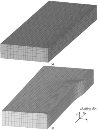
FE simulation of edge rolling should be carried out until the downstream steady-state zone appears, from which a dog-bone profile may be extracted. It follows that the volume of the material to be pushed into the bite zone is substantial. Consequently, the number of elements and the number of time steps that have to be employed easily exceed 18,000 and 1,000 respectively, as illustrated in Fig.
1, taking more than a couple of days on a desktop computer
before the simulation is completed. It is in this regard that
design of an on-line FE model for the prediction of the dog-
bone profile is imperative. The design may be conducted as
follows;
Fig. 1 Original FE mesh selected for process simulation of edge rolling, (a) before rolling, b) after rolling
Step 1.
The target parameter to be considered in process metamorphosis is the dog-bone profile that may be predicted from FE simulation of edge rolling.
As illustrated in Fig. 2, simulation of edge rolling requires a long slab, since the prediction of the dog-bone profile is possible only when the deformation in the bite zone reaches a steady-state. To be computationally efficient, process metamorphosis should lead to achieving the steady- state deformation with a short slab, which may be accomplished as follows.
a) An extrusion-like process is adopted, where the slab would be squeezed into the roll gap by a punch which is in contact with the back end of the slab and travels along the rolling direction with constant speed. The back end is not allowed to be separated from the punch. The roll-slab interface is assumed to be frictionless.
b) The steady-state deformation may be achieved in the roll gap very fast by imposing a special boundary condition
on the line of symmetry at the front end of the slab. The line, which is depicted as line A in Fig. 3, is forced to move along the rolling direction uniformly with the speed V x . The speed may be determined by the condition that the resultant force to be applied to the line is zero.
(a)
(b)
Fig. 2 Process metamorphosis. (a) The original process - edge rolling, (b) the metamorphosed process – a hypothetical process that looks similar to extrusion
Fig. 3 A hypothetical process. The slab is to be pushed
by the punch to pass through the roll gap, with a
special boundary condition applied to the line of
symmetry (line A) at the front end
Step 2.
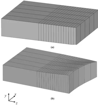
The initial length of the slab to be selected for FE simulation with the hypothetical process should be minimized in order to reduce the number of elements and the number of time steps. Also, the number of the elements in the roll gap should be minimized. Considering that process simulation should be terminated as soon as the front end of the slab exits the roll gap, the guideline selected for the mesh design is as follows:
-The initial length of the slab is 1.25 times as large as the bite zone length.
-Five elements are deployed across the rolling direction.
-One element is deployed across the thickness direction.
-To be capable of representing the dog-bone profile precisely, sixteen elements are deployed across the width direction.
The mesh consists of 80 elements in total, which is 1/225 of the number of the elements in the mesh for edge rolling, as illustrated in Fig. 4. Regarding the number of time steps, 40 steps are selected, which is 1/25 of the number of the time steps required for simulation of edge rolling.
Step 3.
There is a marked difference in the mechanism of forming the dog-bone between the hypothetical process and the original process. On the other hand, the dog-bone profile varies sensitively with roll radius. It may then be concluded that, in order to obtain the same dog-bone profile, the roll radius of the hypothetical process should be different from that of the original process.
A constant may be defined to describe the relation between the two roll radii, as follows.
(1)
where l and l are the roll gap length of the hypothetical process and that of the original process, respectively, R and R are the roll radius of the hypothetical process and that of the original process, respectively, W 1 is the slab width before edge rolling, and W 2 is the slab width after edge rolling.
Fig. 4 On-line FE mesh selected for simulation of the hypothetical process, (a) before rolling, (b) after rolling
It may be assumed that a varies linearly with the reduction ratio, or
(2)
Constants a
1and a
2, which have been determined from a series of FE simulation, are shown in Table 1. Note that the constants may vary with the carbon content and temperature.
It turns out that the plain carbon steel, the flow stress of which is given by Misaka [5], is too soft to withstand the extremity of the boundary conditions imposed on the line A, leading to failure in obtaining the solution convergence.
However, this should not raise any problem, since there are no restrictions regarding the choice of the material for the hypothetical process. The material chosen for the hypothetical process is the one that shows the elastic perflectly-plastic behavior, the yield stress of which is given by
(3)
1 2
1 2
( )
( )
R W W
a l
l R W W
1 2
1 2
1
W W
a a a
W
1 2
1 2
1
W W
Y b b
W
Constants b
1and b
2, which have been determined from a series of FE simulation, are shown in Table 1. Note that the constants may vary with the carbon content and temperature.
Application.
A variety of process conditions are considered to examine the validity of the on-line model, as described in Table 1. The computation time required for simulation with the on-line FE model is less than 1.0 second. Predictions from the on-line FE model are in excellent agreement with predictions from FE simulation of edge rolling, as illustrated in Fig. 5 and Fig. 6.
Table 1 Process conditions selected for edge rolling
5. Concluding remarks
In this paper, the three steps to design an on-line FE model, which are process metamorphosis, mesh design, and process variable design, are described in detail.
Fig. 5 Dog-bone profiles. Prediction from the on-line FE model, prediction from FE simulation of edge rolling. Process conditions are given by A1-L in Table 1
Fig. 6 Dog-bone profiles. Prediction from the on- line FE model, prediction from FE simulation of edge rolling. Process conditions are given by case C in Table 1
It is demonstrated that an on-line FE model that would replace an original FE model can be derived from process metamorphosis, in a step by step manner.
It may be deduced from the present investigation that on- line FE models for the prediction of the target parameters other than dog-bone profile can also be easily found. In part II of this paper, the applicaation of this technology in other metal forming process would be examined.
FEM Online FEM
Case
V
Rmpm C (%)
T (°C)
W
1(mm) W
2(mm) R (mm)
H
1(mm)
1 2
1
W W W
a Y
(GPa)
A1-S 194 0.034 1200 1640.2 1623.0 1045 192 0.011 3.00 0.2
A2-S 194 0.034 1200 1235.4 1210.0 1045 214.6 0.021 2.89 0.36
C 150 0.037 985 1095.2 1072.0 460 143 0.021 2.88 0.37
A3-S 194 0.034 1200 950.5 928.0 1045 280 0.024 2.86 0.41
B 170 0.2 1100 1350.0 1290.0 850 160 0.044 2.64 0.75
A1-L 194 0.034 1200 1640.2 1523.0 1045 192 0.072 2.35 1.18
A3-L 194 0.034 1200 950.5 881.0 1045 280 0.073 2.33 1.21
A2-L 194 0.034 1200 1235.4 1130.4 1045 214.6 0.085 2.20 1.40
1 2 1 2