Air Pollutants Tracing Model using Perceptron Neural Network and Non-negative Least Square
Suk-Hyun Yu
†, Hee-Yong Kwon
††ABSTRACT
In this paper, air pollutant tracing models using perceptron neural network(PNN) and non-negative least square(NNLS) are proposed. When the measured values of the air pollution and the contribution concentration of each source by chemical transport modeling are given, they estimate and trace the amount of the air pollutants emission from each source. Two kinds of emissions data are used in the experiments : CH4 and N2O of Geumgo-dong landfill greenhouse gas, and PM10 of 17 areas in Northeast Asia and eight regions of the Korean Peninsula. Emission values were calculated using pseudo inverse method, PNN and NNLS. Pseudo inverse method could be used for the model, but it may have negative emission values. In order to deal with the problem, we used the PNN and NNLS methods. As a result, the estimation using the NNLS is closer to the measured values than that using PNN. The proposed tracing models have better utilization and generalization than those of conventional pseudo inverse model.
It could be used more efficiently for air quality management and air pollution reduction.
Key words: Air Pollution Tracing Model, Perceptron, Non-negative Least Square
※ Corresponding Author : Hee-Yong Kwon, Address : 310, Arikwan, Anyang Univ., Anyang 5-dong, Manan- gu, Anyang-si, Gyeonggi-do, 430-714, Korea,
TEL : +82-031-467-0878, FAX : +82-031-463-1249, E-mail : [email protected]
Receipt date : Oct. 24, 2013, Revision date : Nov. 8, 2013 Approval date : Nov. 15, 2013
††
Dept. of Information & Communications Engineering, Anyang Univ.
(E-mail: [email protected])
††
Dept. of Computer Science Engineering, Anyang Univ.
1. INTRODUCTION
After the Industrial Revolution, air pollution has been increasing due to rapid industrialization and urbanization. Air pollutants can cause phys- ical damage to the human body directly and/or indirectly and it can lead to social and economic loss.
Air pollutants can be divided into primary pol- lutants such as sulfur dioxide(SO
2), carbon mon- oxide(CO), and lead(Pb), and secondary pollutants such as nitrogen dioxide(NO
2), particulate mat- ter(PM10), and ozone(O
3). The contamination of primary pollutants have been reduced by the air
pollution regulatory policy intensively promoted since the 1990s. The contamination of secondary pollutants, however, have been increased due to automobiles, industrial activities, and the con- struction sites[1]. Among them, greenhouse gases causing a large number of complaints and PM10 being harmful to the human body should be man- aged with particular emphasis.
The greenhouse gases could be generated by energy industries, industrial processes, agri- culture, waste, land use, and forestry. In order to reduce the gases, IPCC (Intergovernmental Panel on Climate Change) has presented the guideline for greenhouse gas inventories[2,3].
In Korea, in order to survey a landfill, not only
FOD (First Order Decay) method presented by
IPCC, but also greenhouse gases direct measur-
ing method using flux chamber to derive the val-
ue of its reaction constant, k has been used. It,
however, has a defect in that measuring time is
limited, emissions from landfill surface are not
uniform, and the cost is high. Recently, mainly in
the developed countries, not only FOD method
but also new estimating techniques using micro- climate data around landfills, methane concen- tration and the application of modeling techniques have been studied [4].
PM is a complex mixture of solid and liquid particles that vary in size and composition, and remain suspended in the air. PM10 is defined as particulate matter with a diameter less than 10 μ m. Many health effect studies have shown an as- sociation between exposure to PM10 and increase in daily mortality and symptoms of certain ill- nesses such as asthma, chronic bronchitis, de- creased lung function, and premature death[5].
The social damage cost of the metropolitan area due to particulate matter is estimated to be worth 10 trillion won per year [6].
It is important to estimate the exact emissions in order to reduce the damage of all of these pollutants. In Korea, the city of Seoul constructs a national and international emissions database with the research results of the National Institute of Environmental Research[7,8], Moon et al. cal- culate yellow dust emissions associated with the 5 expression of experience and the ADAMS mod- el equations of National Weather Service re- spectively, and calculate and check the PM10 concentrations using WRF_CMAQ.
Henze et al. at the University of Columbia evaluated PM2.5 emissions in the United States using the GOES-Chem Adjoint model[9], Jacob, Harvard University's Professor, evaluated the global CO emissions using MOPITT satellite da- ta[10]. Domestic PM10 is largely affected by a long-range trans-boundary movement in the Northeast Asia region. Thus, for the fine metro- politan air quality management, it requires a complex analysis for the long-distance movement and local sources. For this, it is essential to ob- tain accurate domestic and Northeast Asia emis- sions data.
In this paper, we have collected the INTEX-B emission inventory data of greenhouse gases in
Geumgo-dong landfill and East Asia region.
Then, we propose an air pollutant sources tracing model to estimate greenhouse gases, CH
4, N
2O and PM10. The purpose of research is the esti- mation of emissions of each source with green- house gas data in domestic and East Asia regions. When measured emissions and con- tribution concentrations of each source by a chemical transport modeling are given, it is an optimization problem finding emission values of each source to minimize the error between the measured values and the estimated ones.
In this paper, three methods were studied.
First, emissions of each source was estimated using the pseudo inverse method. There was a small error between the measured emissions and the estimated ones, but the negative estimate of the emissions occurred, so it should be improved.
Second, we use PNN which shows excellent learning capability, given a target value. PNN learning may have negative emissions, so we im- prove the network adding the learning conditions to limit the negative weights. Then we resolve the pseudo inverse method's defect of negative emission problem. Third, in order to reduce the error between measured emission values and the ones calculated by the proposed PNN, the NNLS method was applied. The results calculated by the NNLS are closer to the measured emissions than those of the PNN.
In section 2, we describe the proposed models.
Experimental results are shown in section 3, and concluded in section 4.
2. PROPOSED TRACING MODEL
2.1 The definition of air pollutant tracing model
Given measured emissions and contribution
concentrations of each source by a chemical
transport modeling, the model should estimate
emissions of each source. It is an optimization
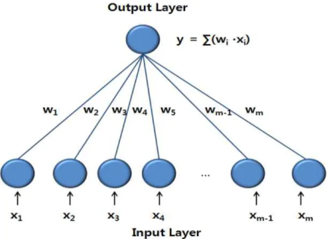
Fig. 1. Single Layer Perceptron.
problem finding emission values, Q of each source to minimize the error between the meas- ured values and the estimated ones, can be ex- pressed as (1).
× (1)
( : measured emissions, : contribution concentrations by chemical transport modeling,
: emissions of each source)
Also, each term in (1) can be defined as follows.
′(2) (
: measured value, : measuring site,
: site number)
(3)
(
: contribution concentration of meaur- ing value of site, : number of measure- ments, : number of sources)
′(4) (
: emission value of source, : number of sources)
2.2 Emission estimation using Pseudo Inverse Method
Emission estimation problem can be regarded as estimating to fit with measured values
, which are described in (1). It can be solved as follows (5), and is called pseudo inverse meth- od[12].
(5)
However, there exist negative emissions when the pseudo inverse method is applied with the problem. As the negative values are not compat-
ible with the physical world, it should be com- pensated with non-negative values. Thus we in- troduce PNN and NNLS to overcome the limi- tation of pseudo inversion.
2.3 Emission estimation using Perceptron Neural Network (PNN)
The human brain performs calculation to react to an external stimulus of environmental factors by the physical interconnection of the cells called neurons. Neural Network model is an intelligent system which mimics the human brain's neu- rons[11].
Neural network for the emission estimation
problem can be designed with single-layer per-
ceptron network model, which consists of input
layer and output layer of neurons. Contribution
concentrations, are the input for the input
layer, measured values are presented as the
output, target for the output layer. With these
neural networks, the weights connecting input
layer with output are learned, which ultimately is
the emissions of each source. Figure 1 shows the
proposed neural network model. In the figure, an
output pattern is calculated by summation of the
results of multiplication weights( ) with con-
tribution concentration input( ). The differ-
ence between the output and the measured val-
ues(C) is the error for the pattern. PNN regulates
the weights ( ) with the error and learns the emission values of each source. It is important to include a condition that when a weight has neg- ative value, it should be limited with non-neg- ative value. Because the weights are emission values and there is no negative emission in the real world, it can not be negative. Neural network learning with such condition can improve the negative emission calculated by pseudo inverse method. Table 1 shows the parameters of the proposed PNN.
Table 1. Neural Network Parameter
2.4 Emission estimation using Non-negative Least Square (NNLS)
Using PNN, the negative emission of pseudo inverse method could be resolved. However, NNLS with constraints of (6) is more efficient than PNN for the problem. In (6), denotes measured emissions, denotes contribution con- centrations obtained by the chemical transport modeling, and estimated emissions which should be calculated. Namely, NNLS estimates that approximates an to , so it is suitable for the problem. Also, it implements the rule that negative weights should not be allowed like PNN [13-21].
║ ║ subject to ≥ (6)
3. EXPERIMENTS AND RESULTS
3.1 Experimental environment
There are two experimental data : one is do- mestic data for Geumgo-dong landfill greenhouse gas, and the other is global data for PM10 of 17 areas in Northeast Asia and 8 regions of the Korean Peninsula. Greenhouse gas measurements
were performed on the bank which separates the landfill into two areas, active and inactive, at in- tervals of 10m. 5 data sets are collected. The emission gases to be estimated are CH
4and N
2O.
Second experiments are performed for the global PM10 which is affected by long-distance travel over the Northeast Asia territories. For more accurate calculations, we use INTEX-B emission inventory. INTEX-B is an emissions data to the region since 2001, reflecting the rapid growth in Asia to complement the TRACE-P emissions in 2000. Target year is 2006, the 0.5 °
× 0.5 ° spatial resolution of emissions data of which target is anthropogenic sources, the target materials are SO
2, NOx, CO, NMVOC, OC, BC, PM10, and PM2.5. Source categories are Power, Industry, Residential, and Transportation. There are included PM10 and PM2.5, but excluded NH
3and biological combustion emissions from the calculation compared with the TRACE-P emissions.
In this paper, we use the PM10 emissions of 17 regions and countries of the Northeast Asia and 8 domestic areas in INTEX-B[22].
3.2 Experimental results
Three experiments are performed : pseudo in- verse method, perceptron neural network(PNN), non-negative least square(NNLS).
As a result, pseudo inverse method has the smallest error between measured emissions and the model's output, but it has a negative emission problem. To deal with the problem, we use PNN and NNLS. Eventually, NNLS has smaller error than PNN, and is the most appropriate method among the three.
Figure 2 and Figure 3 are the estimating re-
sults of the proposed three methods for the
greenhouse gases, CH
4and N
2O. Local case 1 ~
5 are the 5 measurement sets in September 2010
of Daejeon Geumgo-dong landfill. Figure 4 is the
estimating results of the proposed three methods
for the PM10 emissions of 17 regions and coun-
Table 2. RMSE of Three Methods (CH
4, N
2O)
Table 3. RMSE of Three Methods (PM10) tries of the Northeast Asia and 8 domestic areas.
Global case 1 ~ 4 are the 4 PM10 emission data in January 2008, May, August, and October, one for each season. In the graph, x-axis denotes measurement site, y-axis denotes emission.
Legends are measured values , pseudo inverse method, NNLS, and PNN respectively.
In addition, Table 2 and Table 3 shows the RMSE of the proposed three methods' estimation.
4. CONCLUSION
In this paper, we propose air pollutant tracing models by minimizing the error between the measured values and the estimated ones, when measured emissions and contribution concen- trations of each source by a chemical transport modeling are given. The study is conducted with pseudo inverse method, PNN, and NNLS to esti- mate the emissions. Pseudo inverse method esti- mates emissions closest to the measured ones, but there exist negative emissions. We introduce PNN and NNLS to overcome the problem. As a result, both two method resolve the negative emission problem but NNLS'error is smaller than PNN. So NNLS is the best model for emission tracing.
The proposed air pollutant tracing model does
not need expensive equipment or personnel com-
mitments for modeling, so it is efficient in terms
of cost and time. However, it has a defect that
the minimum or maximum value of the measured
emissions may fail to be found. Thus, in order to
be an effective model, not only reducing the error
between measured emissions and estimated ones
but also finding the trends in the emissions is
eventually required.
0 5 10 15 20 25 30 35 40 0
0.005 0.01 0.015
NNLS vs Other Tracing Models with local case 1 (CH4)
Measurement Area Number
Estimation Value
MEASUREMENT VALUE PINV NNLS PERCEPTRON
(a) local case 1
0 5 10 15 20 25 30 35 40
0.004 0.006 0.008 0.01 0.012 0.014 0.016 0.018 0.02 0.022
NNLS vs Other Tracing Models with local case 2 (CH4)
Measurement Area Number
Estimation Value
MEASUREMENT VALUE PINV NNLS PERCEPTRON
(b) local case 2
0 5 10 15 20 25 30 35 40
2 3 4 5 6 7 8 9 10
11x 10-3 NNLS vs Other Tracing Models with local case 3 (CH4)
Measurement Area Number
Estimation Value
MEASUREMENT VALUE PINV NNLS PERCEPTRON
(c) local case 3
0 5 10 15 20 25 30 35 40
4 5 6 7 8 9
10x 10-3 NNLS vs Other Tracing Models with local case 4 (CH4)
Measurement Area Number
Estimation Value
MEASUREMENT VALUE PINV NNLS PERCEPTRON
(d) local case 4
0 5 10 15 20 25 30 35 40
2 4 6 8 10 12
14x 10-3 NNLS vs Other Tracing Models with local case 5 (CH4)
Measurement Area Number
Estimation Value
MEASUREMENT VALUE PINV NNLS PERCEPTRON
( e) local case 5
Fig. 2. NNLS vs. Other Methods with local data(CH
4).
0 5 10 15 20 25 30 35 40 3
4 5 6 7 8 9
10x 10-4 NNLS vs Other Tracing Models with local case 1 (N2O)
Measurement Area Number
Estimation Value
MEASUREMENT VALUE PINV NNLS PERCEPTRON
(a) local case 1
0 5 10 15 20 25 30 35 40
2 4 6 8 10 12
14x 10-4 NNLS vs Other Tracing Models with local case 2 (N2O)
Measurement Area Number
Estimation Value
MEASUREMENT VALUE PINV NNLS PERCEPTRON
(b) local case 2
0 5 10 15 20 25 30 35 40
0.5 0.6 0.7 0.8 0.9 1 1.1 1.2 1.3 1.4
1.5x 10⁻³ NNLS vs Other Tracing Models with local case 3 (N2O)
Measurement Area Number
Estimation Value
MEASUREMENT VALUE PINV NNLS PERCEPTRON
(c) local case 3
0 5 10 15 20 25 30 35 40
0.8 0.85 0.9 0.95 1 1.05 1.1 1.15 1.2
1.25x 10⁻³ NNLS vs Other Tracing Models with local case 4 (N2O)
Measurement Area Number
Estimation Value
MEASUREMENT VALUE PINV NNLS PERCEPTRON
(d) local case 4
0 5 10 15 20 25 30 35 40
1 1.1 1.2 1.3
1.4x 10⁻³ NNLS vs Other Tracing Models with local case 5 (N2O)
Measurement Area Number
Estimation Value
MEASUREMENT VALUE PINV NNLS PERCEPTRON
(e) local case 5
Fig. 3. NNLS vs. Other Methods with global data(N
2O)
0 5 10 15 20 25 40
60 80 100 120 140 160 180 200 220
NNLS vs Other Tracing Models with global case 1
Measurement Area Number
Estimation Value
MEASUREMENT VALUE PINV NNLS PERCEPTRON
(a) global case 1
0 5 10 15 20 25
20 30 40 50 60 70 80 90 100 110 120
NNLS vs Other Tracing Models with global case 2
Measurement Area Number
Estimation Value
MEASUREMENT VALUE PINV NNLS PERCEPTRON
(b) global case 2
0 5 10 15 20 25
20 40 60 80 100 120 140 160 180 200 220
NNLS vs Other Tracing Models with global case 3
Measurement Area Number
Estimation Value
MEASUREMENT VALUE PINV NNLS PERCEPTRON
(c) global case 3
0 5 10 15 20 25
40 60 80 100 120 140 160 180
NNLS vs Other Tracing Models with global case 4
Measurement Area Number
Estimation Value
MEASUREMENT VALUE PINV NNLS PERCEPTRON