1. Introduction
Inter-tidal flat is a shoreline landform resulting from the deposition process of suspended sediments by tidal action. Tidal flat in a river mouth or coastal bay creates an estuary ecosystem that provides valuable habitat for thousands of species. Furthermore, the inter-tidal zone plays very important role in assimilating vast amount of discharges of untreated sewage, industrial wastes, and many other polluted materials from the inland (Odum, 1989). Although the geomorphology of inter-tidal flat changes constantly due to tidal actions, the rate of change has been accelerated by human activities such as
reclamation, embankment, coastal developments, and inland watershed managements. Continuous monitoring of the morphologic changes of tidal flats and the coastal line is important for the conservation of such susceptible ecosystems, as well as the management practises in fishery industry and coastal development planning.
Satellite remote sensing has been an attractive alternative for mapping and monitoring the environmental and morphological status of the coastal area (Cracknell, 1999; Welch et al., 1992). Multi- temporal satellite images have been utilized to analyze the morphologic changes in coastal areas and wetlands where the seasonal variations were significant (Frihy et
Topographic Relief Mapping on Inter-tidal
Mudflat in Kyongki Bay Area Using Infrared Bands of Multi-temporal Landsat TM Data
Kyu-Sung Lee and Tae-Hoon Kim Department of Geoinformatic Engineering, Inha University
Abstract : The objective of this study is to develop a method to generate micro-relief digital elevation model (DEM) data of the tidal mudflats using multi-temporal Landsat Thematic Mapper (TM) data. Field spectroscopy measurements showed that reflectance of the exposed mudflat, shallow turbid water, and normal coastal water varied by TM band wavelength. Two sets of DEM data of the inter-tidal mudflat area were generated by interpolating several waterlines extracted from multi-temporal TM data acquired at different sea levels. The waterline appearing in the near-infrared band was different from the one in the middle-infrared band. It was found that the waterline in TM band 4 image was the boundary between the shallow turbid water and normal coastal water and used as a second contour line having 50cm water depth in the study area. DEM data generated by using both TM bands 4 and 5 rendered more detailed topographic relief as compared to the one made by using TM band 5 alone.
Key Words : Tidal Flat, Multi-Temporal, TM, DEM, Coastal Zone.
Received 10 May 2004; Accepted 11 June 2004.
al., 1994; Lunetta and Balogh, 1999). Construction of three dimensional terrain surfaces in shore areas has been the main interest of several studies, which were related to the coastal change detection. There have been a few attempts to construct DEM data of the shoreline areas using various types of multi-temporal satellite images (Ahn et al., 1989; Chen and Rau, 1998; Ryu et al., 2000; Hickey et al., 2000).
The objective of this study was to develop a methodology to construct a three-dimensional topographic data of inter-tidal zone using multi-temporal satellite images. In this study, we attempted to enhance the procedure for extraction of the waterlines between seawater and land by applying the spectral characteristics near the land-water boundary features.
2. Methods
1) Study Area and Data Used
The western coast of the Korean peninsula has one of the largest tidal flats in the world. Inter-tidal flats in this region have proved to be sources of productive shellfish industry and the habitat for thousands of adopted species. However, the economic and environmental values of the tidal flats have been steadily overwhelmed by the urgent needs of land caused by rapid industrialization and population growth. Kyongki Bay, located in the central part of the western coastal region, is famous for its vast area of well-developed mud dominant inter-tidal flats. The bay area encompasses the mouths of several rivers including the Han and the Imgin Rivers, which have annually discharged a great amount of sedimentation from the area of 42,000km
2watershed. The Seoul and Incheon metropolitan areas, having a population of approximately twenty million people, are attached to Kyongki Bay and have a continual impact on the biophysical and chemical
conditions of the tidal mudflats. During the last few decades, a large area of the tidal mudflats has been converted to industrial, transportation, agricultural, and residential uses. Land reclamations, sedimentation discharges, and the high dynamics of tidal currents would be major forces, which can bring about the geomorphologic changes in the tidal mudflat zone.
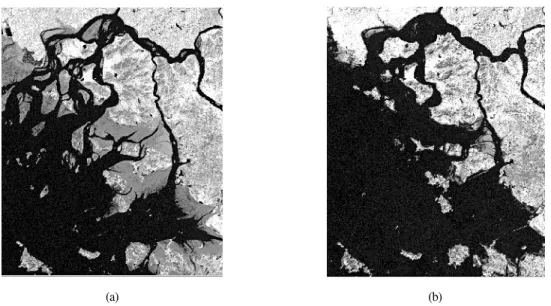
Although the inter-tidal zone in Kyongki Bay has been surveyed to some extent, the exact size and morphology of the flat has not been determined because of the high variation of exposed lands due to the large tidal range. The maximum tidal range between low tide and high tide is close to 9 meters in Kyongki Bay. Fig. 1 shows the images of two Landsat TM bands of the Kyongki bay covering approximately 65×75km
2in which the upper portion of the bay is the mouth of the Han River passing through the Seoul metropolitan area and other two rivers flowing from North Korea. TM images in Fig. 1, which were captured at low tide in 1991 and at high tide in 1999, show the size variation of the exposed tidal flat. Although Landsat satellite has a sun-synchronous orbit passing the study area at approximately the same local time, the tidal flats appearing on the TM images vary greatly according to the sea level at the time of data acquisition.
In this paper, the primary data analysis is focused on the inter-tidal zone near the Yongjong Island. This study site includes a vast area of well-developed, mud dominant, and gently sloped inter-tidal flats due to the large tidal difference of 9 meters (Hong, 1998). Because of the recent large-scale construction of the Incheon International Airport that was built on the west-side tidal flat of the island, it is a great concern to investigate any possible morphological and biochemical changes on the remaining tidal mudflats.
Multiple scenes of Landsat TM data were obtained to
include the large range of tidal elevations in the area
(Table 1). Five TM scenes were used to create the
terrain surface of the tidal flat and the exact sea levels
corresponding with the TM data acquisition time were obtained from the tidal records measured at the Incheon harbor. Since the exact sea level is different from place to place within the large area, such as Kyongki bay, we used 20 additional sea level data that were provided by the National Oceanographic Research Institute (NORI).
The additional tidal elevation values were either directly measured at local stations near the Incheon Harbor or indirectly estimated by the NORI.
2) Waterline Extraction and DEM Generation
In this study, the waterlines between land and water body were delineated from multi-temporal satellite
images collected at different sea levels and used as contour lines to generate DEM data of the inter-tidal zone. Extraction of waterline in tidal flat has been one of the crucial tasks in such cases as well as in other applications of coastal remote sensing. It is, however, not simple to delineate the exact boundary between the land and water body over the tidal flat area. The near-infrared band of SPOT HRV and Landsat TM data were frequently used to extract the waterline (Chen and Rau, 1998; Manavalan et al., 1993) while other middle- infrared band (Frazier and Page, 2000) was also used. As Ryu et al. (2002) pointed out, however, the exaction of waterline between water body and landmass can be varied by several factors including the tidal condition, the turbidity, the grain size, and the remnant surface water.
As can be seen in Fig. 1, the size and shape of the inter-tidal flat vary greatly according to the large range of tidal heights. Since we know the exact sea level at the time of TM data acquisition, the waterline extracted from the TM image can be treated as an elevation contour. If there are multiple satellite images obtained at different sea levels, the three-dimensional surface of the Fig. 1. Kyongki Bay on two TM band 5 images covering approximately 65×75km
2area. The exposed inter-tidal flats are quite
different between the two TM images taken at low tide in 1991 (a) and at high tide in 1999 (b).
(a) (b)
Table 1. List of multi-temporal Landsat TM data obtained at different sea level.
Satellite Acquisition date/ Sea level (M.S.L.) local time at Incheon Harbor Landsat 5 May 21, 1999 / 10:49 244.8cm Landsat 5 Dec. 28, 1998 / 10:49 158.2cm Landsat 5 June 16, 1997 / 10:40 65.1cm Landsat 7 June 30, 1999 / 11:03 -221.3cm Landsat 5 Mar. 2, 1999 / 10:50 -408.6cm
Satellite Acquisition date/ Sea level (M.S.L.)
local time at Incheon Harbor
tidal flat could be generated by these contour lines. To delineate the waterline between seawater and exposed mudflat, it has been common to use a single band image of near-infrared band or a combination of two bands, such as vegetation index. From the visual interpretation of the TM colour composite as well as a single band display, we found that the waterline boundaries were different by the TM spectral bands (Lee et al., 2001).
Fig. 2 shows the exposed inter-tidal flats on two infrared bands of TM data captured at low tide on June 20, 1999.
The waterlines on the near-infrared image of band 4 did not correspond with the lines seen on the middle- infrared image of band 5.
Unlike the sand beach and rocky shore where the spectral reflectance between land and seawater is distinct, it is not quite straightforward to delineate the exact boundary between water body and mudflat. The inter-tidal lands on the western coast of Korean Peninsula are mostly composed of thick layers of mud and clay and the surfaces are fairly flat with little topographic relief, which makes it difficult to distinguish between the mudflats and seawater on satellite images (Ryu et al., 2002). Shallow tidewater flowing over the tidal flat becomes very turbid as they mix with the thick layers of clay, silt and sand particles. The turbidity
decreases as the water depth increases. Tidal water becomes clear when it reaches beyond a certain depth.
From the previous study on the spectral measurement of the mudflat under different surface conditions, it was found that the TM spectral reflectance varied by the turbidity that was directly related to the water-depth near the waterline on the tidal flat (Lee et al., 2001). Detailed description about the laboratory and field measurements of spectral reflectance and turbidity can be referred to Lee et al. (2001). To define the relationship between the turbidity and the water depth, water samples were collected at different water depth. At each water depth, spectral reflectance were measured and two or three water samples were collected. The turbidity was measured by using a DRT-15CE portable turbidimeter in which the turbidity was measured in the nephelometric turbidity units (NTU).
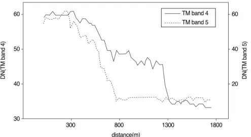
The waterlines were extracted from both TM band 4 and band 5 images by spatial convolution filtering. A Sobel edge detector was applied to create edge lines between the seawater and mudflat (Jensen, 1996). After initial waterlines were extracted, they were edited and cleaned up to assure an accurate representation of the elevation at the time of data acquisition for each TM scene. Fig. 3 shows profiles of digital number (DN) Fig. 2. Different waterline boundaries on two TM bands over the inter-tidal mudflat near the Yongjong Island. Two TM images
were captured at low tide on June 20, 1991: band 4 (a) and band 5 (b).
(a) (b)
value for a transact line, as shown in Fig. 2, crossing from the exposed tidal flat to seawater. Although the sudden drops of DN value in the profile may indicate the boundaries between the tidal flat and water body, their locations are quite distant between the two bands. The waterline boundary in TM band 5 should be at 800m while the waterline that appeared on TM band 4 was around 1,300m. Because the TM bands 4 and 5 data were captured at the same time, one or both of the waterlines may not be indeed the true boundary between
the mudflat and seawater.
Two sets of contour maps were derived from multiple sets of TM data to generate DEM data. The first set of contour map has only five waterlines extracted from TM band 5 images of different tidal levels. The second contour map has ten waterlines in which two waterlines were extracted from both bands 4 and 5 of each TM data set. The waterline extracted from the TM band 5 was given an elevation value according to the sea level.
Since tidal height is different from place to place, we cannot use a single elevation value to each contour line.
To solve the problem, tidal elevation values, which had been corrected by NORI, of 20 stations within the study site were interpolated and the elevation values corresponding to the contour line were extracted. As a result, the waterline derived from TM image does not represent a single elevation value and rather include slight different elevation values according to the location. The elevation value assigned to the waterline from band 4 was 50cm lower than sea level (will be explained later). Each contour map was used to generate separate DEM data for the inter-tidal mudflat area using the interpolation scheme suggested by Hutchinson Fig. 4. Location of 50 reference points, which were selected
from the coastal topographic map to compare with the DEM data generated from this study.
Fig. 3. DN value profile of a transact (shown in Fig. 2) crossing from the exposed mudflat to seawater, obtained from band 4 and band 5 of the same TM scene.
60
50
40
30
60
40
20
DN(TM band 4) DN(TM band 5)
300 800 1300 1800
distance(m)
Yongjong Island
TM band 4
TM band 5
(1989).
After two sets of DEM data were constructed with a 10m grid size, the relative accuracy of each DEM data was then compared by using 50 reference points selected the 1:35,000-scale coastal topographic map (Fig. 4). The coastal area topographic map produced by the NORI in 2000 shows the reference points where the exact elevation was measured by in situ surveying.
3. Results and discussions
As explained by the previous study, spectral reflectance near the waterline shows distinct pattern of reflectance curve at various water depth (Lee et al., 2001). The spectral reflectance near the waterline zone varies as a function of water depth. The exposed mudflat showed the highest spectral reflectance as compared to other samples covered by various depths of tidewater.
Spectral reflectance of shallow seawater is influenced by complex interactions of several parameters including water depth, substrate reflectance, and suspended sediments and dissolved substances (Ryu et al., 2002;
Bierwirth et al., 1993). The spectral reflectance measurements near the waterline showed that the actual boundary between the exposed tidal flat and seawater is very likely to be seen at the middle-infrared spectrum (TM bands 5 and 7) rather than at the near-infrared spectrum (TM band 4).
The waterline-like boundary seen in the TM band 4
image is not a true waterline and may be somewhere between very turbid water and normal coastal water.
The turbidity of tidewaters tends to be inversely proportional to the water depth above the mudflats (Fig.
5). Density of suspended sediments activated from the surface of mudflat decreases as the depth of water increases. Tidewaters moving at shallow depth have more interaction with clay and silt particles on the surface of the mudflat and, therefore, have higher turbidity than rather deep tidewaters. When the tidewater has a certain depth above the mudflat, it appears to have almost the same turbidity as normal coastal water. In TM band 4 wavelengths (760 - 900nm), the reflectance of the tidewater at about 50cm depth showed significantly lower reflectance while the exposed mudflat and the very turbid shallow waters were not much different from each other. The boundary between the mudflat and seawater appearing in the TM band 4 was the borderline between the normal coastal water and the high-turbid shallow water (between A and B in Fig. 5).
In the middle-infrared spectrum of TM bands 5 and 7, the exposed mudflat still shows relatively high reflectance while the water samples show very low reflectance regardless of the water-depths. Therefore, the true waterline separating seawater from the mudflat should be seen at middle-infrared wavelength and can be found in TM band 5 or 7 images (A in Fig. 5). As reported by Ryu et al. (2002), however, the waterline extracted from TM band 5 is greatly influenced by the
Fig. 5. Cross-sectional view of tidewater interacting with the surface of a mudflat. The turbidity of tidewater is inversely proportional to the water depth above the mudflat: A is the waterline boundary appearing in TM band 5 and B is the waterline boundary appearing in TM band 4.
water
A d B
High turbidity
Tidal Mudflat
remnant water and might not correspond to A where the remnant water is significant. The distance between A and B may vary according to the slope gradient of the tidal flat surface. Horizontal distance between the waterlines seen in band 5 (A) and band 4 (B) could be several hundred meters at a flat area having a very gentle topographic relief. On the other hand, the two lines may be very close to each other at a tidal zone having very steep slope.
Assuming that the waterline appearing in the TM band 4 is the borderline between the normal coastal water and the high-turbid shallow water, the next question would be the water depth along the line. If we know the exact water depth under the boundary appearing in TM band 4 image, we could use it as another contour line having different elevation value.
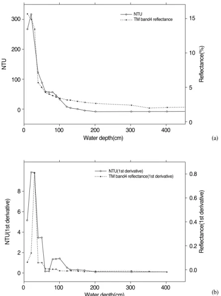
Fig. 6-a shows the relationship between the two variables (turbidity and spectral reflectance of TM band Fig. 6. Relationship of tidewater turbidity and spectral reflectance at TM band 4 as a function of water depth. At about 50cm water
depth, both turbidity and reflectance remain steady at the study site.
0 100 200 300 400
8
6
4
2
0
0.8
0.6
0.4
0.2
0.0 300
200
100
0
NTU
15
10
5
0
0 100 200 300 400
Water depth(cm)
Reflectance(%)
Water depth(cm)
NTU(1st derivative) Reflectance(1st derivative)
NTU
TM band4 reflectance
NTU(1st derivative)
TM band4 reflectance(1st derivative)
(a)
(b)
4 wavelength) and water depth. As mentioned before, the two variables (turbidity and spectral reflectance) are highly correlated (r = 0.975). While turbidity and the reflectance decrease quickly at shallow water depth, they are relatively steady beyond 50cm water depth.
Such a relationship can be seen effectively by applying the first derivative of each variable (Fig. 6-b). At a depth of more than 50cm, both turbidity and reflectance do not change much and remain low value. Therefore, the waterline-like boundary seen in TM band 4 is in fact the
line of about 50cm water depth, which is the boundary between the high turbid shallow water and the normal coastal water.
The marginal water depth, in which the upper level of tidewater does not mix with the surface materials of the mudflat, is about 50cm at the study site. The waterline- like boundary seen in TM band 4 is indeed the line of about 50cm water depth, which is the boundary between the high turbid shallow water and the normal coastal water. As a result, we used the waterline extracted from
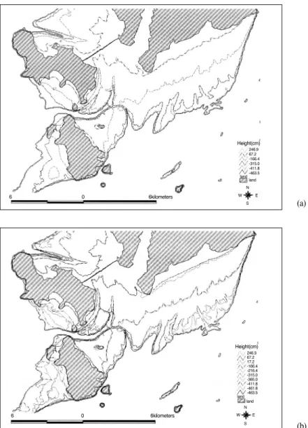
Fig. 7. Comparison of the two sets of waterline contour map extracted from only TM band 5 (a) and from both TM bands 4 and 5 (b).
Height(cm)
60 6kilometers
landland
N
S E W
246.9 67.2 -166.4 -315.0 -411.8 -463.5
60 6kilometers
Height(cm) 246.9 67.2 17.2 -166.4 -216.4 -315.0 -365.0 -411.8 -461.8 -463.5 land
land N
S E W
(a)
(b)
TM band 4 as contour line having an elevation value 50cm lower than the sea level at the time of the data acquisition. The waterline extracted from TM band 5 image has an elevation value of the corresponding sea level. Fig. 7 shows the two sets of finalized contour maps prepared for the DEM generation.
Interpolating the waterlines extracted from band 5 alone and from both band 4 and band 5 generated two sets of DEM data. As seen in Fig. 7, the three- dimensional surfaces of the mudflats were better represented by the DEM data created by using both band 4 and 5 images. In particular, the southwestern tidal flats of the two islands show micro-scale topographic relief with the contour map using both TM band 4 and 5. The DEM data using both TM bands 4 and 5 waterlines also showed more detailed topographic features, such as small tidal creeks and shoals.
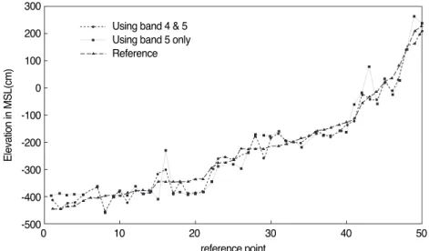
The relative accuracy estimated by the reference points also supported the result of visual interpretation.
Fig. 8 compares the elevations values derived from the two DEM datasets and the 50 reference points measured on the coastal topographic map. The elevation values derived from the DEM data using two bands were closer
to the reference values with low root mean squared error of 30.6cm, as compared to the 47.0cm RMSE with the DEM data using band 5 only.
Because of the distinct spectral characteristics along the waterline of the tidal mudflats, the waterlines extracted from the bands 4 and 5 of the same TM scene behaved as separate contour lines having different elevations. If we can further relate the depth and turbidity of shallow tidal waters with their spectral characteristics, we might be able to extract more contour lines from other bands (visible and other infrared wavelength) of multi-spectral image acquired at the same time and construct the DEM data with a fewer number of temporal data sets.
Although the inter-tidal flats in Kyongki Bay have been greatly altered by human activities as well as by coastal deposition and erosion, we do not know the exact size and shape of the inter-tidal flat areas. The DEM data generated by multi-temporal TM data can provide not only the exact size of tidal flat area but also the volume of the flats. Since Kyongki Bay has a relatively large tidal range and a very dynamic tidal action, the volumetric changes in the tidal flat zone can Fig. 8. Comparison of the elevation values derived from the two DEM surfaces with the 50 known values of the reference points
on the coastal topographic map.
300 200 100 0 -100 -200 -300 -400 -500
Elevation in MSL(cm)