Analysis of M-WiMAX Uplink Capacity with Receive Beamforming and Adjacent Channel Interference from WCDMA Downlink

Analysis of M-WiMAX Uplink Capacity with Receive Beamforming and Adjacent Channel Interference from WCDMA Downlink

YuPeng Wang* Associate Member, KyungHi Chang* Lifelong Member

ABSTRACT

In this paper, we analyze the M-WiMAX UL capacity limits under 2-Tier cell layout, considering the effects of random user position, path loss models, fading channel and adjacent channel interference from WCDMA system. In order to make the analysis approximate to the practical system capacity, we propose a MCS-based capacity analysis method considering the effects of PER requirement and the utilized MCS levels in M-WiMAX system. The proposed MCS-based method is validated through a system-level Monte Carlo simulation. Furthermore, a comparison between the conventional Shannon method and the proposed MCS-based method is presented and the optimum cell radius is suggested.

Key Words : M-WiMAX, WCDMA, Capacity, Receive Beamforming, Adjacent Channel Interference

* 인하대학교 정보통신대학원 이동통신연구실 ([email protected])

논문번호：KICS2007-10-468, 접수일자：2007년 10월 12일, 최종논문접수일자 : 2008년 02월 20일

Ⅰ. Introduction

The 2500 – 2600 MHz band has been identified as an additional spectrum band that administrations may choose to make available for IMT-2000

. As a result, the ACI (Adjacent Channel Interference) from the WCDMA system to the M-WiMAX system, which is operating in the adjacent band of the WCDMA system, should be mitigated without results in performance degradation of the M-WiMAX system.

RxBF (Receive Beamforming) is a well-known technique to mitigate interference and to increase the received signal power. In [2]-[4], some work is done considering the capacity issues in point to point link with RxBF and other multiple antenna technology. In addition, some methodologies to analyze the system capacity are described in [5], considering the independent effect of path loss, shadowing, fading channel, user position under 1-Tier cell layout. However, little research work is drawn to analyze the capacity issue of M-WiMAX system with RxBF in UL (Up-Link), considering the joint effect of path loss, fading channel,

random user position, adjacent channel interference from WCDMA system, and the practical PER (Packet Error Ratio) and MCS (Modulation and Coding Scheme) requirements. Therefore, we analyze lower and upper capacity limits in M-WiMAX UL with RxBF in the M-WiMAX BS, based on the conventional Shannon and the proposed MCS-based methods, when ACI coming from WCDMA system. We validate the proposed MCS-based capacity analysis through system-level Monte Carlo simulation and make a comparison with the conventional Shannon method.

The remainder of this paper is organized as follows. In section II, we introduce the capacity analysis procedure based on the Shannon equation and our proposed MCS-based method, considering the random user position, practical path loss models, fading channels and ACI from the WCDMA BS.

Section III presents the numerical procedures to

calculate the M-WiMAX UL capacity limits for

both methods and the system-level Monte Carlo

simulation environment which we use to validate

our proposed MCS-based analysis method. Simulation

results and discussions are described in section IV. Conclusions are drawn in section V.

Ⅱ. Methodologies of Capacity Analysis in M- WiMAX System with ACI from WCDMA System In this section, we derive the capacity limits in M-WiMAX UL with RxBF based on the conventional Shannon equation and the proposed MCS-based method, considering the effects of random user position, path loss models in [1], fading channel, and ACI from WCDMA system. To take the effect of ACI into consideration, the conventional SIR (Signal-to-Interference Ratio) metric has been changed to SINR (Signal-to- Interference and Noise Ratio).

In the proposed MCS-based method, the system PER (Packet Error Rate) requirement and available MCS (Modulation and Coding Scheme) level are considered in order to analyze the capacity in a more practical way. To make the analysis simple and avoid the effect of scheduling, we assume only user is active in each sector.

2.1 Random User Position

For analytical convenience, we assume that the cell shape is approximated by a circle of radius

be mutually independent and uniformly distributed in their corresponding cells. Thus, the PDF (Probability Density Function) of the UEs polar coordinates (r,

) relative to their BS are as (1) and (2)．

0 2 0 0

2( )

( ) ,

( )

r

p r r R R r R

R R

= − ≤ ≤

− (1)

1 , 0 2

p_θ

2 θ π

= π ≤ ≤ 　 　(2)

R₀

corresponds to the closet distance that the UE can be away from the BS antenna, and is assumed to be 1 m in this paper.

2.2 Path Loss Models

To analyze the M-WiMAX system capacity in a more practical way, we utilize different path loss models for the cases of BS to BS and UE to BS [1], rather than only one single free space path loss model.

The dual-slope LOS (Line of Sight) model is

used for the case of BS to BS, considering a more realistic propagation environment [1]. This model assumes free-space propagation until the breakpoint d

After the breakpoint, the attenuation is increased due to diffraction and reflection effects.

The BS to BS path loss model is as (3).

10

10 10

40.7 20log ( ), 1 ( ) 40.7 20log ( ) 40log ( ),

BS BS

break

break break

d d d

PL dB

d d d d

−

+ ≤ ≤

=⎨ ⎧ ⎩ − + > (3)

where d is the distance of BSs in meters, and the breakpoint is calculated as

λ

tx break

h d

= 4 ⋅

⋅

(4) where h

and h

are the heights (over the reflecting surface) of the transmitter and the receiver (both are 6 meters in this paper); and

is the wavelength.

For the case of UE to BS, we used the path loss model for the vehicular test environment [1].

It is

(

)

10

( ) 40(1 4 10 ) log ( ) 18 log ( ) 21 log ( ) 80,

UE BS b b

PL dB h r h

f

−

= − ×

Δ ⋅ − ⋅ Δ

+ ⋅ + (5)

where

is the difference between the BS antenna height and the average building height, for which the value of 6 is used. In the analyses, the average building height is set to 24 m and r (specified in kilometers) is the horizontal distance between the BS and the UE

≥ 100 m f is the operating frequency in megahertz, which is set to 2600 MHz in this paper.

If the UE to BS separation is less than 30 meters, the free space pass loss model of (6) is applied.

( ) 20 log( ) 20 log( ) 32.44

= ⋅

+ ⋅

+ (6)

If the UE to BS separation is between 30 to 100

meters, the LOS or NLOS (Non Line of Sight)

model is selected randomly, the probability P(LoS)

for LoS, increases with decreasing separation, r,

as follows.

1 2

1 2

2 1

2

1

( ) 0

r R R r

P LoS R r R

R R

r R

⎧ ≤

⎪ −

= ⎪ ⎨ ⎪ − ≤ ≤

⎪ ≥

⎩ (7)

where R

is 30 meters and R

2.3 Multipath Fading Channel with RxBF in M-WiMAX BS

In this paper, we assume the M-WiMAX BS has N

has N

=1 antenna. We assume each transmit and receive antenna pair has independent Rayleigh fading, and the channel keeps constant over several OFDM symbols. In general, we can decompose the fading coefficient matrix H using the SVD (Singular Value Decomposition) operation [6] and [7].

=

H UΛV (8)

where U, Λ, V are matrices of dimension N

×

, N

× N

, N

× N

, respectively. The matrices

=

, and VV

= V

The matrix Λ = [

] is a diagonal matrix with diagonal entries being equal to the nonnegative square roots of the eigenvalues of either H

, and thus, are uniquely determined. Generally, the rank of the channel matrix H is determined by min (N

, N

) [8]. Therefore, after SVD operation only one nonnegative eigenvalue

exists in the case of

=1, and the channel eigenvalue

_{is as}

2 1 NR

i i

λ

=

= ∑ (9)

where h

is the independent Rayleigh fading coefficient between the UE antenna and the i

antenna element in the BS. From the assumption of independent Rayleigh fading on each antenna pair, we find that

_follows the Chi-Square distribution with 2N

degrees of freedom and the PDF is as (10).

/ 2 1 / 2 /2

1 , for 0

2 ( / 2) ( ; )

0 for 0

k x

k x e x

k f x k

x

⎧ − − >

⎪ Γ

= ⎨⎪⎩ ≤

⁽¹⁰⁾

where k is the freedom of Chi-square distribution, and Γ(z) denotes Gamma function as (11).

( ) (

1)!, is Integer

Γ = − (11)

2.4 Capacity Derivation

In this sub-section, we obtain the M-WiMAX UL capacity limits, considering the random user position, practical path loss models, fading channel and the effect of ACI from WCDMA system. In this paper, we consider the M-WiMAX and WCDMA BS are in the co-sited deployment.

The fading channel frequency response on the

1 2 0

=

N i kn

k n N

n

H h e

− −π⋅

∑

(12) where N

is the FFT size, h

is the channel response for the n

sample. Due to the assumption that the channel keeps constant over-several OFDM symbols, all the subcarriers have the same channel power gain, which is equal of the eigenvalue

of the channel covariance matrix HH

.

If we assume the equal power allocation is used in the M-WiMAX UE, all the subcarriers will have the same received SINR values. The received SINR considering ACI from WCDMA BS, with distance r to the target M-WiMAX BS can be written as

2 2

int int

( ) ( ) ( )

( )

r

r sc

AWGN er ACI AWGN er ACI

P r N P r SINR r

P P N P P

λ λ

σ σ

= = ⋅

+ + + +

(13)

where

( )

is the received power and the inter-cell interference power from other M- WiMAX UEs on each subcarrier, considering the UE to BS path loss model as (5)-(7);

received ACI power from WCDMA BS on each subcarrier, considering the coupling loss between two system BS antennas; σ

is the AWGN background noise; and N is the number of data subcarrier.

From (13), we observe that

and ^σ

are

independent of the UE position. Thus, we can

obtain the max SINR on each subcarrier with distance r when the least

is received by target M-WiMAX BS, which means all the interfering M-WiMAX UE have the furthest distance to the target M-WiMAX BS, and vice versa. Based on this observation, we can get the upper and lower capacity limits in M-WiMAX UL according to the positions of the interfering M-WiMAX UEs. The actual UL capacity of M- WiMAX system should lie between the upper and lower limits.

Due to the existence of ACI, we used SINR instead of SIR to calculate Shannon capacity. The Shannon capacity C ( )

on one single subcarrier considering the UE with distance r to the target BS is as follows.

sc 2 2

int 0

C ( ) log (1 1 _r( ) ) ( ; )

AWGN er ACI

r B P r x f x k dx

N σ P P

∞

= + ⋅ ⋅

+ +

∫

₍₁₄₎

where

^{( ; )} is the PDF of the Chi-square distribution, and B is the effective bandwidth of M-WiMAX system.

Considering the random position of the desired UE, we can write the M-WiMAX UL capacity as

2 0 0 sc

2

2 2

0 0

int 0

C ( ) ( )

= log (1 1 ( ) ) ( ; ) ( )

R

UL r

R

r r

AWGN er ACI

C p N r p r drd

B P r x f x k p r p dxdrd

P P

π θ π

θ

θ σ θ

∞

= ⋅ ⋅

+ ⋅ ⋅

+ +

∫ ∫

∫ ∫ ∫

(15) From (15), we find that the M-WiMAX UL capacity depends on the system effective bandwidth

of data subcarrier N.

Due to the assumption of arbitrary small BER and no limit on the modulation level in Shannon capacity calculation, there will be some difference between the calculated Shannon capacity and the actual system capacity. Therefore, we derived the MCS-based method considering the system PER requirement and the available MCS levels.

According to the definition of throughput, the MCS-Based system capacity can be written as

Re 0 _

(1 )

i i

n

q MCS MCS

i UL MCS

Sym

PER N P N

C T

=

− ⋅ ⋅

= ∑

(16)

where PER

is the system PER requirement; n is the number of MCS levels available in the system;

MCSi

P

is the probability of utilizing the i

MCS level;

is the number of information bits on each subcarrier per symbol when the i

MCS level is used, which is determined by the modulation level and coding rate; and T

is the effective OFDM symbol time. The utilization probability of the i

MCS level can be calculated as (17).

_ 1

_

_ 1

_ 2

0 0 2

2

0 0 0 int

= ( ( )) ( )

= [ 1 ( )

( ; )

tar MCSi

i SC Rx

tar MCSi

tar MCSi tar MCSi R SINR

MCS SINR SINR sc

R SINR SINR r

AWGN er ACI

P f SINR r d SINR drd

P r x

P P

f x k

π

π

θ σ

+

+

∞

⋅ ⋅

+ +

⋅

∫ ∫∫

∫ ∫∫ ∫

( ) ]

dxp r p drdr _θ θ

⁽¹⁷⁾ where

is the PDF of the received SINR on one subcarrier with distance r to the target BS;

and

+

are the target received SINR values for the i

and (i+1)

MCS level, respectively.

Ⅲ. Simulation Environment and Parameter Setting

3.1 Numerical Analysis

In (15) and (17), we observe that multiple integrations are involved in the calculation. Thereby, it is very difficult to get the closed form equation for them, especially for (17) where arbitrary integration period may be used. Thus, we build a numerical analysis platform to calculate the capacity limits.

The procedure of numerical analysis is shown in Fig. 1.

3.2 System-level Monte Carlo Simulation In this paper, we consider 2-Tier deployment layout for both victim M-WiMAX system and interfering WCDMA system. And there are total of 57 sectors in 19 hexagonal cells [9]. All the UEs in the 19 hexagonal cells have random positions, which follow the uniform distributions as (1) and (2).

In system-level Monte Carlo Simulation, we assume

the ideal sectorized antennas are used and the

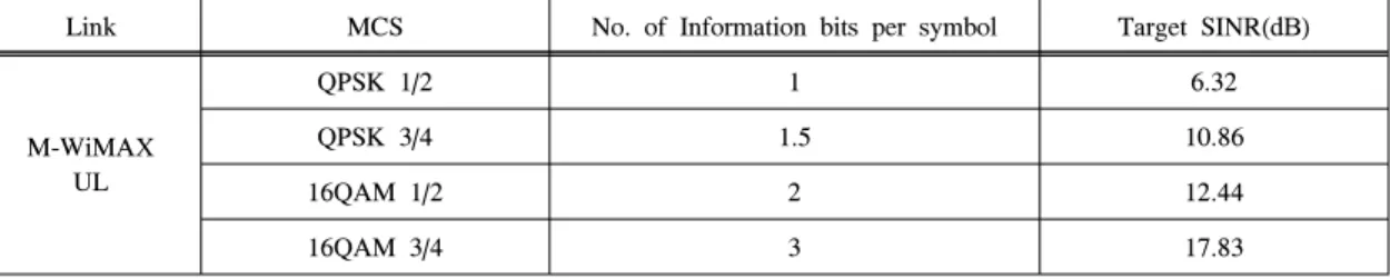
Link MCS No. of Information bits per symbol Target SINR(dB)

M-WiMAX UL

QPSK 1/2 1 6.32

QPSK 3/4 1.5 10.86

16QAM 1/2 2 12.44

16QAM 3/4 3 17.83

Table 1. MCS level, the number of information bits per symbol and the target SINR values for each MCS level in the M-WiMAX UL.

Fig. 1 Numerical analysis procedures for both Shannon and MCS-based capacity limits.

channel is known to the M-WiMAX BS, therefore we can calculate the RxBF weighting factor for each subcarrier based on the SVD operation of (8).

The receiver weighting factor on the k

subcarrier can be chosen as

2

( )

/

k k

k H H

k k k k AWGN PTx

θ

= σ ×

+

W H V a

V H H V

(18)

where H

, V

are the generated matrices by the SVD operation on the kth subcarrier; P

is the transmitted power; and a(

) is the array factor with the desired signal DoA (Direction of Angle) [10].

Thus, the received SINR on the k

subcarrier can be calculated as

10

10 2 int

10 ( ) ( )

10 ( ) ( ) ( )

s

i PL

H

Tx k k

k PL

H

i i k AWGN ACI k k

SINR P

P P

θ θ

θ θ σ

′

⋅ ⋅

=

′

⋅ + +

∑

w a a w

a a w w w

(19)

where PL

is the path loss of the desired UE in dB value; PL

UE to the target BS; and

is the DoA of the

interfering UE to the target BS.

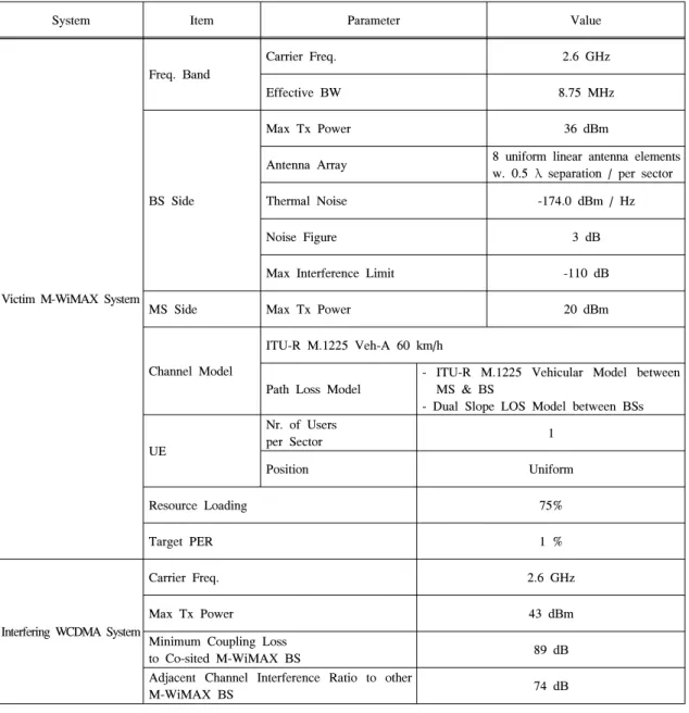
Table I shows the available MCS levels, number of information bits per modulated symbol and the target SINR values for each MCS level in the M-WiMAX UL, which will be used in both numerical analysis and Monte Carlo simulations. Furthermore, the parameters for the system-level Monte Carlo simulation are shown in Table II.

Ⅳ. Numerical Results and Discussion

In this section, we show the capacity limits obtained by the Shannon equation and MCS-based methodology in the M-WiMAX UL through numerical analysis for the cases of SISO (Single Input and Single Output) and RxBF, considering random user position, practical path loss models, fading channel, and ACI coming from WCDMA DL under a 2-Tier cell layout. In addition, the system-level Monte Carlo simulation results are also presented.

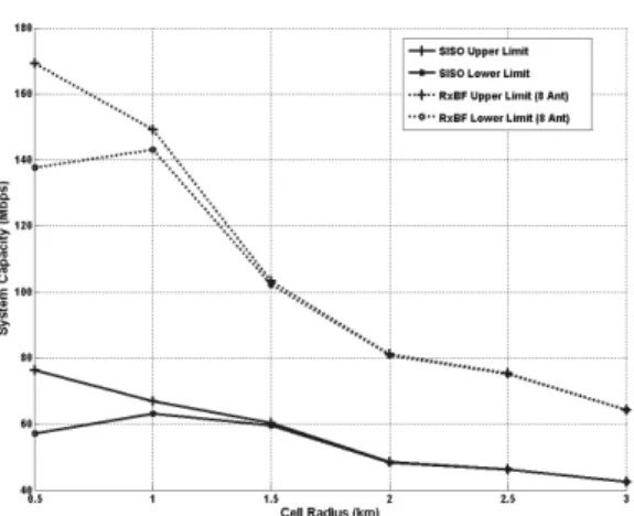
Figure 2 presents the Shannon capacity with single and 8 antennas in the M-WiMAX BS based on (15).

From this figure, we find that the upper limit on the Shannon capacity decreases as the cell radius

Besides, the maximum lower limit appears at the

cell radius of 1 km for both cases. At the same

time, we find that the RxBF induced capacity

gain is inverse proportional to the cell radius and

the difference between the two limits approaches

closer as the cell radius increases, which is due

to the fact that the effect of inter-cell interference

gets smaller and smaller as the cell radius gets

System Item Parameter Value

Victim M-WiMAX System

Freq. Band

Carrier Freq. 2.6 GHz

Effective BW 8.75 MHz

BS Side

Max Tx Power 36 dBm

Antenna Array 8 uniform linear antenna elements w. 0.5

separation / per sector

Thermal Noise -174.0 dBm / Hz

Noise Figure 3 dB

Max Interference Limit -110 dB

MS Side Max Tx Power 20 dBm

Channel Model

ITU-R M.1225 Veh-A 60 km/h

Path Loss Model

- ITU-R M.1225 Vehicular Model between MS & BS

- Dual Slope LOS Model between BSs

UE

Nr. of Users

per Sector 1

Position Uniform

Resource Loading 75%

Target PER 1 %

Interfering WCDMA System

Carrier Freq. 2.6 GHz

Max Tx Power 43 dBm

Minimum Coupling Loss

to Co-sited M-WiMAX BS 89 dB

Adjacent Channel Interference Ratio to other

M-WiMAX BS 74 dB

Table 2. Parameters for system-level Monte Carlo simulation.

larger and larger.

In Fig. 3, the MCS-based capacity limits and the Monte Carlo simulation results are shown for the case of single and 8 antennas configuration in the M-WiMAX BS. We observe that the capacity obtain by Monte Carlo simulation nearly lies in the middle of the capacity limits based on (16) for both cases. That is, in Monte Carlo simulation all the interfering M-WiMAX UEs are random located in their respective sectors, and the target BS suffers nearly moderate inter-cell interference between that in the cases of upper and lower

limits. Furthermore, all the capacity limits are inversely proportional to the cell radius. As the cell radius increases, we also see that the capacity gain induced by RxBF decreases.

Comparing the limits of Shannon and MCS-

based capacities, very huge difference are observed

due to the impractical assumption of the arbitrary

small BER and no limits on modulation level in

Shannon capacity calculation. Under these assumptions,

the UEs which are near to the target BS will be

assigned very high modulation level and high system

throughput is obtained. To avoid the impractical

Fig. 2 Upper and lower capacity limits in the M- WiMAX UL based on the Shannon equation for both SISO and RxBF with 8 antennas.

Fig. 3 Comparison between the capacity limits of the proposed MCS-based method and the Monte Carlo simulation in the M-WiMAX UL.

assumptions in the Shannon capacity, the MCS- based capacity method is proposed, which is also validated by the Monte Carlo simulation results in Fig 3.

Ⅴ. Conclusions

In this paper, we analyze capacity limits of the M-WiMAX UL, i.e., upper and lower limits with adjacent channel interference from WCDMA DL, based on the conventional Shannon equation and a proposed MCS-based method. Due to the existence of adjacent channel interference, the conventional SIR metric is replaced by the SINR metric to take ACI effect into consideration. Furthermore, the proposed MCS-based capacity analysis method

is validated through system-level Monte Carlo simulation. We find that the capacity limits obtained from the Shannon equation has very huge difference compared with the simulation results under the practical environments, due to the impractical assumptions in Shannon equation. Therefore, the proposed MCS- based method is more proper to analyze the practical system capacity than the conventional Shannon method. In addition, we vary the cell radius to find the optimum cell coverage. Considering the max lower capacity limit obtained by Shannon method, the potential of higher modulation utilization in the M-WiMAX UL, and the fact that small cell coverage causes more handovers, it is better to choose 1 km as the cell radius. From both analytical and simulation results, we observe that RxBF with 8 antennas results in at least 80%

increase on the system capacity with the cell radius of 1 km.

References

[1] ITU Spectrum SWG Sharing Studies WP8F 443-E, Aug. 2006.

[2] M. S. Alouini and A. J. Goldsmith, “Capacity of Rayleigh fading channels under different adaptive transmission and diversity-combining techniques,” IEEE Trans. Veh. Technol., vol.48, no.4, pp.1165-1181, July 1999.

[3] H. Bolsckei, D. Gesbert, and A. J. Paulraj, “On the capacity of OFDM-based spatial multiplexing systems,” IEEE Trans. Commun., vol.50, no.2, pp.225-234, Feb. 2002.

[4] A. Goldsmith, S. A. Jafar, N. Jindal and S.

Vishwanath, “Capacity limits of MIMO channels,”

IEEE J. Select Areas Commun., vol.21, no.5,

pp.684-701, June 2003.

[5] M. S. Alouini and A. J. Goldsmith, “Area spectral efficiency of cellular mobile radio systems,”

IEEE Trans. Veh. Technol., vol.48, no.4, pp.

1047-1066, July 1999.

[6] R. A. Hom and C. R. Johnson, Matrix Analysis.

Cambridge, U.K.: Cambridege Univ. Press, 1985.

[7] P. Lancaster and M. Tismenetsky, The Theory

Academic, 1985.

[8] S. K. Jayaweera, and H. V. Poor, “Capacity of multiple-antenna systems with both receiver and transmitter channel state information,” IEEE

2709, Oct. 2003.

[9] Cdma2000 Evaluation Methodology, Revision 0, Dec. 2004.

[10] YuPeng Wang, SangJun Ko, and KyungHi Chang, “Adjacent interference analysis between M- WiMAX OFDMA/TDD and WCDMA FDD system in the 2.6 GHz band - Part II:

Adjacent interference analysis with smart antenna in M- WiMAX system,” Journal of Korea

32, no.6, pp. 588-599, 2007. 06.

왕 우 붕 (YuPeng Wang) 준회원

2004년 7월 동북대학교 통신공학 과 (공학사)

2006년 7월 인하대학교 정보 통 신대학원 (공학석사)

2006년 9월~현재 인하대학교 정 보 통신대학원 박사과정

<관심분야> Mobile-WiMAX / 3GPP LTE 시스템, Radio Resource Management, Relay Network, MIMO Technique, UWB

장 경 희 (KyungHi Chang) 종신회원

1985년 2월 연세대학교 전자공학 과 (공학사)

1987년 2월 연세대학교 전자공학 과 (공학석사)

1992년 8월 Texas A & M Univ., EE Dept. (Ph.D.)

1989년~1990년 삼성종합기술원 주임연구원

1992년~2003년 한국전자통신연구원, 이동통신연구소 무선전송방식연구팀장 (책임연구원)

2003년~현재 인하대학교 정보통신대학원 부교수

<관심분야> 4세대 이동통신 및 3GPP LTE 무선전송방

식, WMAN 및 DMB 시스템 무선전송기술,

Cognitive Radio, Cross-layer Design, Cooperative

Relaying System, RFID / USN Systems.