Journal of the Korean Society of Surveying, Geodesy, Photogrammetry and Cartography Vol. 32, No. 6, 625-635, 2014
http://dx.doi.org/10.7848/ksgpc.2014.32.6.625
Strip Adjustment of Airborne Laser Scanner Data Using Area-based Surface Matching
Lee, Dae Geon1) · Yoo, Eun Jin2) · Yom, Jae-Hong3) · Lee, Dong-Cheon4)
Abstract
Multiple strips are required for large area mapping using ALS (Airborne Laser Scanner) system. LiDAR (Light Detection And Ranging) data collected from the ALS system has discrepancies between strips due to systematic errors of on-board laser scanner and GPS/INS, inaccurate processing of the system calibration as well as bore- sight misalignments. Such discrepancies deteriorate the overall geometric quality of the end products such as DEM (Digital Elevation Model), building models, and digital maps. Therefore, strip adjustment for minimizing discrepancies between overlapping strips is one of the most essential tasks to create seamless point cloud data. This study implemented area-based matching (ABM) to determine conjugate features for computing 3D transformation parameters. ABM is a well-known method and easily implemented for this purpose. It is obvious that the exact same LiDAR points do not exist in the overlapping strips. Therefore, the term “conjugate point”
means that the location of occurring maximum similarity within the overlapping strips. Coordinates of the conjugate locations were determined with sub-pixel accuracy. The major drawbacks of the ABM are sensitive to scale change and rotation. However, there is almost no scale change and the rotation angles are quite small between adjacent strips to apply AMB. Experimental results from this study using both simulated and real datasets demonstrate validity of the proposed scheme.
Keywords : LiDAR Strip Adjustment, Surface Matching, Sub-pixel Accuracy, Accuracy Assessment
625 ISSN 1598-4850(Print) ISSN 2288-260X(Online) Original article
Received 2014. 11. 28, Revised 2014. 12. 08, Accepted 2014. 12. 16
1) Department of Geoinformation Engineering, Sejong University, Korea (E-mail: [email protected]) 2) Member, Department of Geoinformation Engineering, Sejong University, Korea (E-mail: [email protected]) 3) Member, Department of Geoinformation Engineering, Sejong University, Korea (E-mail: [email protected])
4) Corresponding Author, Member, Department of Geoinformation Engineering, Sejong University, Korea (E-mail: [email protected])
This is an Open Access article distributed under the terms of the Creative Commons Attribution Non-Commercial License (http://
creativecommons.org/licenses/by-nc/3.0) which permits unrestricted non-commercial use, distribution, and reproduction in any medium, provided the original work is properly cited.
1. Introduction
Over the last two decades LiDAR data has been one of the major sources for establishing geospatial information infrastructure including DEM, topographic maps, urban model, GIS database, biomass measurement, and so on.
LiDAR data is collected in strip-wise with multiple strips to scan entire areas. In order to obtain directly geo-referenced point cloud data, laser scanner, GPS and INS are integrated.
However, systematic errors of the individual devices and
inaccurate integration of the multi-sensor (i.e., insufficient system calibration or mounting bias) lead discrepancies in the overlapping areas between adjacent strips. Therefore, strip adjustment to remove or minimize the discrepancies is required to create seamless and compatible data.
Precise calibration requires original observations from GPS/INS and laser range measurements, which are not available to the end users in most cases (Bang et al., 2009;
Kersting and Habib, 2012; Rentsch and Krzystek, 2012).
Instead, 3D coordinates of the LiDAR point data are
Journal of the Korean Society of Surveying, Geodesy, Photogrammetry and Cartography, Vol. 32, No. 6, 625-635, 2014
626
provided. Therefore, the strip adjustment is based on the 3D coordinate transformation between overlapping strips.
The LiDAR script adjustment is similar to independent model adjustment of the aerial triangulation. Therefore, the adjustment parameters are basically composed of scale, translations, and rotations between adjacent strips.
Strip adjustment can be also utilized as internal quality evaluation of the LiDAR data associated with quality of the system calibration even though there is no unique and standard strip adjustment method yet (Habib et al., 2008;
Pfeifer and Bӧhm, 2008; Schenk, 2001). The central issue of the strip adjustment is to define corresponding features and to find locations of the features in the overlapping strips. The corresponding features could be points, lines or planes (e.g., corners, edges or roof facets of buildings). Several studies have carried out to improve LiDAR data quality through the strip adjustment. Crombaghs et al. (2000) proposed a method for reducing vertical discrepancies between overlapping strips. Habib et al. (2008) utilized linear feature matching to solve corresponding problem in the overlapping areas. Kilian et al. (1996) introduced a procedure similar to the aerial photo strip adjustment for detecting discrepancies and improving the compatibility. Maas (2000) suggested a method to establish correspondence by minimizing the normal distances between discrete points in one LiDAR strip and TIN patches in the other strip.
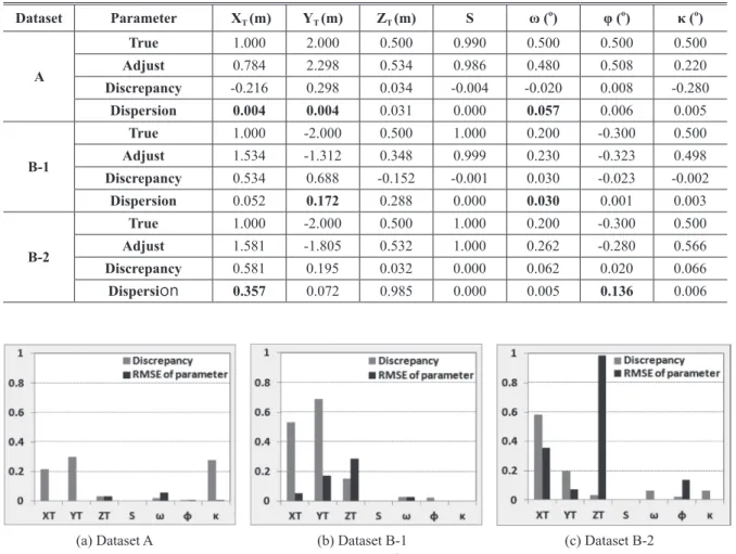
In this paper, the conjugate point features were identified using correlation template matching with sub-pixel accuracy. Template matching takes characteristics of the surface into account. The method finds similarity of the surface patches in the overlapping strips in terms of cross- correlation instead of point-to-point correspondence. The template matching is quite straight forward and easy to implement. The strip adjustment was performed with 3D similarity transformation based on the identified conjugate templates. Finally, the accuracy of the strip adjustment was evaluated by recovery of the discrepancy and RMSE (Root Mean Square Error) of the adjustment parameters, and RMSE of LiDAR point coordinates as well as visual inspection of the profiles after strip adjustment. The results show that the proposed procedure is suitable for airborne LiDAR strip adjustment.
2. Surface Matching for Conjugate Features
2.1 Overview of study
LiDAR strip adjustment procedure consists of three parts:
(1) Determination of the correspondence between overlapping strips
(2) Computation of the adjustment parameters and coordinate transformation
(3) Quality assessment of the parameters and transformed coordinates after adjustment
Correspondence problem is associated with conjugate feature matching. Strip adjustment reduces discrepancies by 3D coordinate transformation. Finally, quality of the strip adjustment is evaluated by checking compatibility of the LiDAR point clouds. Fig. 1 shows the overview of the proposed method.
To find the conjugate points might not be suitable for LiDAR data-derived surfaces because it is almost impossible to identify conjugate points in the overlapping areas. Identification of the distinct points is quite difficult and not reliable due to the irregular nature of the LiDAR footprints. Therefore, it is obvious that most probably the
Fig. 1. Work flow of strip adjustment
Strip Adjustment of Airborne Laser Scanner Data Using Area-based Surface Matching
627 exact same LiDAR points do not exist in the overlapping
strips (Habib et al., 2008). In other words, point-to-point correspondence could not be valid as shown in Fig. 2(a).
Therefore, the term corresponding feature should reflect topographic characteristics of the surface of the interest regions. Template matching depicted in Fig. 2(b) is one of the traditional methods to find similarity between features.
Advantages of the template matching are straight forward, simple and practical to implement while the major drawback is unreliable under scale change, rotations and geometric distortions. In addition, irregularly distributed points are interpolated to create regular grid data. The templates of the reference and target surfaces implicitly represent surface characteristics, and the similarity between surfaces is computed by cross-correlation coefficients. Therefore, template matching is basically not based on point-to-point correspondence but surface-to-surface correspondence.
Some sophisticated matching methods utilize LiDAR data- derived secondary products such as lines or planes that require further processes including extraction of the line features, segmentation of the LiDAR points, grouping and modeling. In consequence, quality of the correspondence would be affected by accuracy of the secondary products.
2.2 Automatic extraction of conjugate features It is not necessary that the matching features are to be specific objects in template matching. However, to find reliable matching features such as well-defined points in the homogeneous areas is difficult. Therefore, to improve matching accuracy and efficiency, selection of the reliable conjugate feature is recommendable. Uniquely identifiable features would be reliable matching candidates to avoid ambiguous or multiple matching. Reliable matching candidates are distinct model key points such as corners of the buildings or other man-made structures. In this study, Canny edge operator (Canny, 1986) and Harrison corner detector (Harris and Stephens, 1988) described from Equation 1 to Equation 4, were used to extract conjugate features. This procedure aims at automatic detection of the most possible conjugate features. Locations of the extracted conjugate feature are to be reference for determining search surfaces.
R = Det(M) – K·[Trace(M)]2 (2)
if (Z(X,Y) ≥ T·Rmax) then corner points at (X,Y) (3)
X = ∑(Rij·X)/ ∑Rij, Y = ∑(Rij·Y)/∑Rij (4)
(5) (i.e., n×m
∑ ∑
= == n
0 i
m j 0 j
ijXiY a ρ
(6)
Y 0 ρ Y X 2 ρ X ρ) ρ (
ρ 2 2 44 24 2 44
4 =
∂ + ∂
∂
∂ + ∂
∂
= ∂
∇
∇
=
∇ (7)
∂ρ/∂X = 0 and ∂ρ/∂Y = 0.
(XT, YT, ZT), (ω, φ, κ)
M T P
+
= (8)
] Z , Y , [X R S
= M , ] Z , Y , [X
= T , ] Z , Y , [X
=
P 2 2 2 T T T T T ⋅ ⋅ 1 1 1 T
ω,φ,κ. (X1, Y1, Z1) (X2, Y2, Z2)
i i
⋅
⋅ + +
=
Z Y X dR dS) (1 dZTT dYT dX Zo
Yo Xo
(9)
. (Xo, Yo, Zo) (i.e. i-1)
∂
∂
∂
∂
∂
∂
∂
∂
∂
∂
∂
∂
=
∑∑ ∑∑
∑∑
∑∑
= =w i
w j w 2
i w
j
w i
w j 1
i w
1 j
2
Y ) Y) ( Z(X, Y )
Y) )( Z(X, X
Y) ( Z(X,
Y ) Y) )( Z(X, X
Y) ( Z(X, X )
Y) (Z(X, M
w
(1)
R = Det(M) – K·[Trace(M)]2 (2)
if (Z(X,Y) ≥ T·Rmax) then corner points at (X,Y) (3)
The coordinates of a corner point in the local window are computed by:
X = ∑(Rij·X )/ ∑Rij, Y = ∑(Rij·Y )/∑Rij (4)
where M is a gradient matrix computed from partial derivatives with respect to X and Y. Z(X,Y) denotes Z-coordinate at (X,Y). w is local window size. K and T denote threshold values. Rij is R value at (i,j) in the local windows.
2.3 Determination of conjugate features
Incorrectly determined conjugate features deteriorate strip adjustment (Pfeifer et al., 2005). Template size and locations of the search surface are significant factors in the Fig. 2. LiDAR point distribution and matching conjugate
features
(a) LiDAR point distribution in overlapping strip
(b) Templates and search surface for matching
Journal of the Korean Society of Surveying, Geodesy, Photogrammetry and Cartography, Vol. 32, No. 6, 625-635, 2014
628
template matching. The size and locations depend on the point density (or average ground distance) and tolerance of the GPS/INS accuracy. The centers of the templates are not necessarily distinct points (e.g., building corners).
However, it is recommended to avoid locating templates in homogeneous areas because to determine the maximum correlation is ambiguous in such area. The cross-correlation in the overlapping strips is computed by Equation 5.
R = Det(M) – K·[Trace(M)]2 (2)
if (Z(X,Y) ≥ T·Rmax) then corner points at (X,Y) (3)
X = ∑(Rij·X)/ ∑Rij, Y = ∑(Rij·Y)/∑Rij (4)
(5) (i.e., n×m
∑∑
= == n
0 i
m j 0 j
ijXiY a ρ
(6)
Y 0 ρ Y X 2 ρ X ρ) ρ (
ρ 2 2 44 24 2 44
4 =
∂ + ∂
∂
∂ + ∂
∂
= ∂
∇
∇
=
∇ (7)
∂ρ/∂X = 0 and ∂ρ/∂Y = 0.
(XT, YT, ZT), (ω, φ, κ)
M T P
+
= (8)
] Z , Y , [X R S
= M , ] Z , Y , [X
= T , ] Z , Y , [X
=
P T 1 1 1T
T T T T 2 2
2 ⋅ ⋅
ω,φ,κ. (X1, Y1, Z1) (X2, Y2, Z2)
i i
⋅
⋅ + +
=
Z Y X dR dS) (1 dZTT dYT dX
Zo Yo Xo
(9)
. (Xo, Yo, Zo) (i.e. i-1)
∂
∂
∂
∂
∂
∂
∂
∂
∂
∂
∂
∂
=∑∑ ∑∑
∑∑
∑∑= =
w i w
j w 2
i w
j
w i w
j 1
i w
1 j
2
Y ) Y) ( Z(X, Y )
Y) )(Z(X, X
Y) (Z(X,
Y ) Y) )(Z(X, X
Y) (Z(X, X )
Y) (Z(X, M
w
(5)
where n and m denote the template size (i.e., n×m), ZT(Xi,Yi) is Z-coordinate at (Xi,Yi) in template, ZM(Xi,Yi) is Z-coordinate at (Xi,Yi) in the matching windows inside of the search surface, ZT and ZTZMZM are averages of the Z-coordinates in template and matching window, respectively.
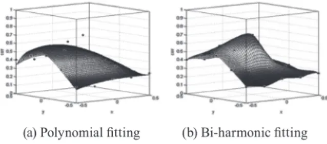
The correlation surfaces were formed by fitting mathematical functions. To choose an appropriate mathematical function is crucial since shape of the surfaces depend on the fitting functions. Fig. 3 shows two correlation surfaces. Fig. 3(a) and Fig. 3(b) are results from 3rd-order polynomial and bi-harmonic fitting in a search window, respectively. Since a conjugate feature with sub-pixel accuracy is to be located near maximum correlation, polynomial fitting using Equation 6 might not be appropriate representation of the correlation surfaces.
Instead, the bi-harmonic function according to Equation 7 renders the correlation surface reasonably compared with polynomial surface.
R = Det(M) – K·[Trace(M)]2 (2)
if (Z(X,Y) ≥ T·Rmax) then corner points at (X,Y) (3)
X = ∑(Rij·X)/ ∑Rij, Y = ∑(Rij·Y)/∑Rij (4)
(5) (i.e., n×m
∑ ∑
= == n
0 i
m j 0 j
ijXiY a ρ
(6)
Y 0 ρ Y X 2 ρ X ρ) ρ (
ρ 2 2 44 24 2 44
4 =
∂ + ∂
∂
∂ + ∂
∂
= ∂
∇
∇
=
∇ (7)
∂ρ/∂X = 0 and ∂ρ/∂Y = 0.
(XT, YT, ZT), (ω, φ, κ)
M T P
+
= (8)
] Z , Y , [X R S
= M , ] Z , Y , [X
= T , ] Z , Y , [X
=
P 2 2 2 T T T T T ⋅ ⋅ 1 1 1 T
ω,φ,κ. (X1, Y1, Z1) (X2, Y2, Z2)
i i
⋅
⋅ + +
=
Z Y X dR dS) (1 dZTT dYT dX Zo
Yo Xo
(9)
. (Xo, Yo, Zo) (i.e. i-1)
∂
∂
∂
∂
∂
∂
∂
∂
∂
∂
∂
∂
=
∑∑ ∑∑
∑∑
∑∑
= =w i
w j w 2
i w
j
w i
w j 1
i w
1 j
2
Y ) Y) ( Z(X, Y )
Y) )( Z(X, X
Y) ( Z(X,
Y ) Y) )( Z(X, X
Y) (Z(X, X )
Y) ( Z(X, M
w
(6)
R = Det(M) – K·[Trace(M)]2 (2)
if (Z(X,Y) ≥ T·Rmax) then corner points at (X,Y) (3)
X = ∑(Rij·X)/ ∑Rij, Y = ∑(Rij·Y)/∑Rij (4)
(5) (i.e., n×m
∑ ∑
= == n
0 i
m j 0 j
ijXiY a ρ
(6)
Y 0 ρ Y X 2 ρ X ρ) ρ (
ρ 2 2 44 24 2 44
4 =
∂ + ∂
∂
∂ + ∂
∂
= ∂
∇
∇
=
∇ (7)
∂ρ/∂X = 0 and ∂ρ/∂Y = 0.
(XT, YT, ZT), (ω, φ, κ)
M T P
+
= (8)
] Z , Y , [X R S
= M , ] Z , Y , [X
= T , ] Z , Y , [X
=
P 2 2 2 T T T T T ⋅ ⋅ 1 1 1 T
ω,φ,κ. (X1, Y1, Z1) (X2, Y2, Z2)
i i
⋅
⋅ + +
=
Z Y X dR dS) (1 dZTT dYT dX Zo
Yo Xo
(9)
. (Xo, Yo, Zo) (i.e. i-1)
∂
∂
∂
∂
∂
∂
∂
∂
∂
∂
∂
∂
=
∑∑ ∑∑
∑∑
∑∑
= =w i
w j w 2
i w
j
w i
w j 1
i w
1 j
2
Y ) Y) ( Z(X, Y )
Y) )( Z(X, X
Y) ( Z(X,
Y ) Y) )( Z(X, X
Y) (Z(X, X )
Y) ( Z(X, M
w
(7)
where n and m are order of the polynomial. aij is a coefficient of the polynomials. ∇2 denotes Laplacian operator that performs sum of the second derivatives of the correlation surface with respect to each variable, X and Y.
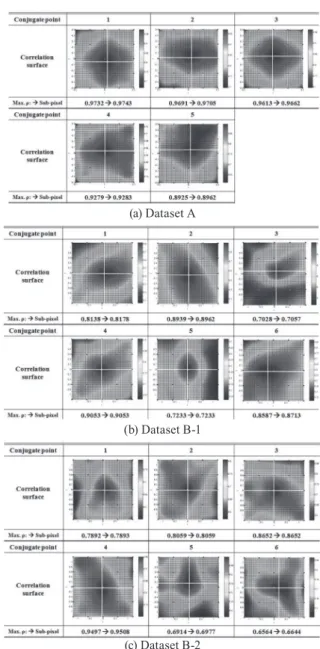
Location of the conjugate feature in each search surface occurs at the maximum correlation. However, the location with maximum correlation might not guarantee to be a conjugate point. Therefore, sub-pixel accuracy should be considered by analyzing correlation surfaces to find accurate matching location. The sub-pixel coordinates of the matching locations could be computed by partial derivatives of the fitting surfaces. i.e., sub-pixel locations of the maximum correlation were estimated by partial derivatives with respect to X and Y where
R = Det(M) – K·[Trace(M)]2 (2)
if (Z(X,Y) ≥ T·Rmax) then corner points at (X,Y) (3)
X = ∑(Rij·X)/ ∑Rij, Y = ∑(Rij·Y)/∑Rij (4)
(5) (i.e., n×m
∑ ∑
= == n
0 i
m j 0 j
ijXiY a ρ
(6)
Y 0 ρ Y X 2 ρ X ρ) ρ (
ρ 2 2 44 24 2 44
4 =
∂ + ∂
∂
∂ + ∂
∂
= ∂
∇
∇
=
∇ (7)
∂ρ/∂X = 0 and ∂ρ/∂Y = 0.
(XT, YT, ZT), (ω, φ, κ)
M T P
+
= (8)
] Z , Y , [X R S
= M , ] Z , Y , [X
= T , ] Z , Y , [X
=
P 2 2 2 T T T T T ⋅ ⋅ 1 1 1 T ω,φ,κ. (X1, Y1, Z1)
(X2, Y2, Z2)
i i
⋅
⋅ + +
=
Z Y X dR dS) (1 dZTT dYT dX Zo
Yo Xo
(9)
. (Xo, Yo, Zo) (i.e. i-1)
∂
∂
∂
∂
∂
∂
∂
∂
∂
∂
∂
∂
=
∑∑ ∑∑
∑∑
∑∑
= =w i
w j w 2
i w
j
w i
w j 1
i w
1 j
2
Y ) Y) ( Z(X, Y )
Y) )( Z(X, X
Y) ( Z(X,
YY)) )( Z(X, XY) ( Z(X, XY))
( Z(X, M
w
and
R = Det(M) – K·[Trace(M)]2 (2)
if (Z(X,Y) ≥ T·Rmax) then corner points at (X,Y) (3)
X = ∑(Rij·X)/ ∑Rij, Y = ∑(Rij·Y)/∑Rij (4)
(5) (i.e., n×m
∑ ∑
= == n
0 i
m j 0 j
ijXiY a ρ
(6)
Y 0 ρ Y X 2 ρ X ρ) ρ (
ρ 2 2 44 24 2 44
4 =
∂ + ∂
∂
∂ + ∂
∂
= ∂
∇
∇
=
∇ (7)
∂ρ/∂X = 0 and ∂ρ/∂Y = 0.
(XT, YT, ZT), (ω, φ, κ)
M T P
+
= (8)
] Z , Y , [X R S
= M , ] Z , Y , [X
= T , ] Z , Y , [X
=
P 2 2 2 T T T T T ⋅ ⋅ 1 1 1 T ω,φ,κ. (X1, Y1, Z1)
(X2, Y2, Z2)
i i
⋅
⋅ + +
=
Z Y X dR dS) (1 dZTT dYT dX Zo
Yo Xo
(9)
. (Xo, Yo, Zo) (i.e. i-1)
∂
∂
∂
∂
∂
∂
∂
∂
∂
∂
∂
∂
=
∑∑ ∑∑
∑∑
∑∑
= =w i
w j w 2
i w
j
w i
w j 1
i w
1 j
2
Y ) Y) ( Z(X, Y )
Y) )( Z(X, X
Y) ( Z(X,
Y ) Y) )( Z(X, X
Y) ( Z(X, X )
Y) ( Z(X, M
w
3. LiDAR Strip Adjustment
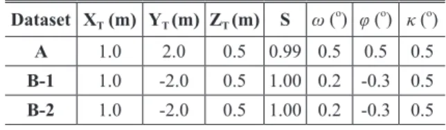
3.1 Computation of adjustment parameters As shown in Fig. 4, relationship between adjacent strips could be determined by 3D similarity transformation having three translations (XT, YT, ZT), three rotation angles (ω, φ, κ) and a scale (S) based on Equation 8.
R = Det(M) – K·[Trace(M)]2 (2)
if (Z(X,Y) ≥ T·Rmax) then corner points at (X,Y) (3)
X = ∑(Rij·X)/ ∑Rij, Y = ∑(Rij·Y)/∑Rij (4)
(5) (i.e., n×m
∑ ∑
= == n
0 i
m j 0 j
ijXiY a ρ
(6)
Y 0 ρ Y X 2 ρ X ρ) ρ (
ρ 2 2 44 24 2 44
4 =
∂ + ∂
∂
∂ + ∂
∂
= ∂
∇
∇
=
∇ (7)
∂ρ/∂X = 0 and ∂ρ/∂Y = 0.
(XT, YT, ZT), (ω, φ, κ)
M T P
+
= (8)
] Z , Y , [X R S
= M , ] Z , Y , [X
= T , ] Z , Y , [X
=
P T 1 1 1T
T T T T
2 2
2 ⋅ ⋅
ω,φ,κ. (X1, Y1, Z1) (X2, Y2, Z2)
i i
⋅
⋅ + +
=
Z Y X dR dS) (1 dZTT dYT dX
Zo Yo Xo
(9)
. (Xo, Yo, Zo) (i.e. i-1)
∂
∂
∂
∂
∂
∂
∂
∂
∂
∂
∂
∂
= ∑∑ ∑∑
∑∑
∑∑= =
w i
w j w 2
i w
j
w i
w j 1
i w
1 j
2
Y ) Y) ( Z(X, Y )
Y) )(Z(X, X
Y) ( Z(X,
Y ) Y) )(Z(X, X
Y) ( Z(X, X )
Y) ( Z(X, M
w
(8)
where
R = Det(M) – K·[Trace(M)]2 (2)
if (Z(X,Y) ≥ T·Rmax) then corner points at (X,Y) (3)
X = ∑(Rij·X)/ ∑Rij, Y = ∑(Rij·Y)/∑Rij (4)
(5) (i.e., n×m
∑∑
= == n
0 i
m j 0 j
ijXiY a ρ
(6)
Y 0 ρ Y X 2 ρ X ρ) ρ (
ρ 2 2 44 24 2 44
4 =
∂ + ∂
∂
∂ + ∂
∂
= ∂
∇
∇
=
∇ (7)
∂ρ/∂X = 0 and ∂ρ/∂Y = 0.
(XT, YT, ZT), (ω, φ, κ)
M T P
+
= (8)
] Z , Y , [X R S
= M , ] Z , Y , [X
= T , ] Z , Y , [X
=
P T 1 1 1T
T T T T
2 2
2 ⋅ ⋅
ω,φ,κ. (X1, Y1, Z1) (X2, Y2, Z2)
i i
⋅
⋅ + +
=
Z Y X dR dS) (1 dZTT dYT dX Zo Yo Xo
(9)
. (Xo, Yo, Zo) (i.e. i-1)
∂
∂
∂
∂
∂
∂
∂
∂
∂
∂
∂
∂
= ∑∑ ∑∑
∑∑
∑∑= =
w i w
j w 2
i w
j
w i w
j 1
i w
1 j
2
Y ) Y) (Z(X, Y )
Y) )( Z(X, X
Y) ( Z(X,
Y ) Y) )( Z(X, X
Y) ( Z(X, X )
Y) ( Z(X, M
w
Fig. 3. Correlation surfaces
(a) Polynomial fitting (b) Bi-harmonic fitting
Fig. 4. 3D coordinate transformation between strips