A Batch Processing Algorithm for Moving k-Nearest Neighbor Queries in Dynamic Spatial Networks

JKSCI

A Batch Processing Algorithm for Moving k-Nearest Neighbor Queries in Dynamic Spatial Networks

1)Hyung-Ju Cho*

*Professor, Dept. of Software, Kyungpook National University, Sangju, Korea

[Abstract]

Location-based services (LBSs) are expected to process a large number of spatial queries, such as shortest path and k-nearest neighbor queries that arrive simultaneously at peak periods. Deploying more LBS servers to process these simultaneous spatial queries is a potential solution. However, this significantly increases service operating costs. Recently, batch processing solutions have been proposed to process a set of queries using shareable computation. In this study, we investigate the problem of batch processing moving k-nearest neighbor (MkNN) queries in dynamic spatial networks, where the travel time of each road segment changes frequently based on the traffic conditions. LBS servers based on one-query-at-a-time processing often fail to process simultaneous MkNN queries because of the significant number of redundant computations. We aim to improve the efficiency algorithmically by processing MkNN queries in batches and reusing sharable computations. Extensive evaluation using real-world roadmaps shows the superiority of our solution compared with state-of-the-art methods.

▸Key words: Spatial databases, Moving k-nearest neighbor query, Batch processing, Dynamic spatial network

[요 약]

위치 기반 서비스(LBS)는 가장 바쁜 시간에 동시에 도착하는 최단 경로 및 k-최근접 이웃 질의를

포함한 다양한 공간 질의를 효과적으로 처리한다. 동시에 도착하는 공간 질의를 빠르게 처리하기 위

한 간단한 해결 방법은 LBS 서버를 추가하는 것이다. 이 방법은 서비스 운영 비용을 많이 증가시킨

다. 최근에는 공유 가능한 계산을 사용하여 일련의 질의를 한꺼번에 모아서 처리하는 일괄 처리 방 법이 제안되었다. 본 연구에서는 교통 상황에 따라 각 도로 구간의 이동 시간이 빈번하게 변하는 동 적 공간 네트워크에서 움직이는 k-최근접 이웃 질의를 한꺼번에 처리하는 방법을 연구한다. 순차적

질의 처리를 기반으로 하는 LBS 서버는 중복 계산으로 인해 한꺼번에 요청이 들어오는 움직이는 k-

최근접 이웃 질의를 효과적으로 처리하지 못한다. 본 연구의 목표는 움직이는 k-최근접 이웃 질의를

한꺼번에 처리하고 공유 가능한 계산을 재사용하여 알고리즘을 효율성을 개선한다. 실제 지도 데이

터를 사용한 실험 평가는 최신 방법보다 제안된 방법이 우수하다는 것을 보여준다.

▸주제어: 공간 데이터베이스, 움직이는 k-최근접 이웃 질의, 일괄 처리, 동적 공간 네트워크

∙First Author: Hyung-Ju Cho, Corresponding Author: Hyung-Ju Cho

*Hyung-Ju Cho ([email protected]), Dept. of Software, Kyungpook National University

∙Received: 2021. 02. 18, Revised: 2021. 03. 31, Accepted: 2021. 03. 31.

Copyright ⓒ 2021 The Korea Society of Computer and Information http://www.ksci.re.kr pISSN:1598-849X | eISSN:2383-9945

I. Introduction

Currently, location-based services (LBSs), such as taxi-calling and ridesharing services, utilize real-time spatial data to find k points of interest (POI) closest to a query point based on the length of the shortest path from the query point to the POI. For example, a taxi client wishes to be served by available taxicabs that can reach them quickly.

LBS servers based on one-query-at-a-time processing often fail to process a large number of simultaneous spatial queries reaching the servers at the peak time. Hence, batch processing algorithms have been introduced to address this critical problem in LBSs [1, 2].

Here, we investigate the batch processing of moving k-nearest neighbor (MkNN) queries in dynamic spatial networks, where the travel time for each road segment changes frequently based on the traffic conditions such as the traffic volume and accidents. MkNN queries in a dynamic spatial network have many potential applications for LBSs, such as ride-hailing and car parks. For example, 14 million Uber trips for ridesharing were completed each day in 2019, demonstrating the significance of scalable and efficient solutions to promptly match Uber cabs with passengers. Another example is real-time parking management, which helps drivers find parking spaces nearest to them. It is often difficult for drivers to find available parking spaces when they reach their destinations.

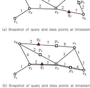
Figure 1 shows two snapshots at timestamps _ and _ of a dynamic spatial network, where a set Q of moving query points and a set P of moving data points are expressed as  ^_ ^and

 ^__, respectively. Note that for the convenience of presentation, two road segments

__ and __ are identified using a double solid line to represent changes in the travel time of these road segments, as shown in Figure 1(b). In Figure 1(a), data point p1 is closest to both q1 and q2 at timestamp ti. However, in Figure 1(b), data

point p1 (p2) is closest to q2 (q1) at timestamp tj. A simple solution for MkNN queries uses a one-query-at-a-time method, which computes k data points that are closest to each query point in Q sequentially. This solution introduces a prohibitive overhead because of redundant network traversal for adjacent query points, despite utilizing efficient kNN search algorithms [3, 4, 5, 6] for retrieving a set of k data points closest to the query point.

(a) Snapshot of query and data points at timestamp _

(b) Snapshot of query and data points at timestamp _ Fig. 1. Example of MkNN queries in a dynamic spatial network

All nearest neighbor (ANN) queries [7] are similar to MkNN queries. However, ANN queries retrieve only one data point closest to each query point q in Q, indicating    for each ∈. Contrarily, MkNN queries retrieve a different number of k data points closest to each query point q. Furthermore, we consider a highly dynamic situation where both the query and data points move freely in dynamic spatial networks. Herein, we propose an efficient algorithm known as BANK for the batch processing of MkNN queries in dynamic spatial networks. The BANK algorithm first groups adjacent query points into a query group and performs batch computation for the query group to avoid

redundant network traversal. To our study, the batch computation approach has not been applied to MkNN queries in dynamic spatial networks;

however, the batch computation of spatial queries has received significant attention.

The primary contributions of this study are listed as follows:

Ÿ We propose an efficient algorithm called BANK for the batch processing of MkNN queries in dynamic spatial networks. To our study, the BANK algorithm is the first to consider the batch processing of MkNN queries in dynamic spatial networks.

Ÿ We present group computation techniques to avoid the redundant computation of network distances for adjacent query points.

Furthermore, we present a theoretical analysis to prove the advantage of the BANK algorithm over one-query-at-a-time methods.

Ÿ We conduct extensive experiments using real- world roadmaps to demonstrate the efficiency of the proposed solution.

The remainder of this paper is organized as follows. In Section II, we review related studies and introduce the background of the study. In Section III, we explain the method for clustering adjacent query points into a query group and present the BANK algorithm for the batch processing of MkNN queries in dynamic spatial networks. In Section IV, we compare the BANK algorithm and its conventional solutions with different setups.

Conclusions are presented in Section V.

II. Preliminaries

1. Related works

Nearest neighbor (NN) queries have been investigated extensively in spatial networks. NN query processing for spatial networks involves a high cost for computing the length of the shortest path between two points, in which graph traversal may be required. Studies regarding NN queries in

spatial networks have presented various techniques to reduce the shortest-path-distance computation.

Papadias et al. [4] introduced the incremental Euclidean restriction (IER) and incremental network expansion (INE). IER is based on the assumption that the length of the shortest path between two points cannot be less than their Euclidean distance. INE involves network expansion from the query point in a manner similar to Dijkstra’s algorithm and examines the data points in the sequence encountered. The distance browsing (DisBrw) algorithm [8] uses the spatially induced linkage cognizance index, which stores the shortest path distance between every pair of vertices. The route overlay and association directory (ROAD) [3]

algorithm hierarchically partitions the spatial network and precomputes the shortest path distance between border vertices within each partition, where border vertices of a partition are the vertices connecting to other partitions. The G-tree [6]

partitions the spatial network; however, it differs from the ROAD in terms of the tree structure and searching paradigm. The V-tree [5] employs a hierarchical structure similar to that of the G-tree;

it identifies border nodes at the boundaries of subgraphs. Efficient techniques are used to answer kNN queries by maintaining the lists of data points closest to the border nodes. Abeywickrama et al. [9]

performed a thorough experimental evaluation of several kNN search algorithms for spatial networks, including G-tree [6], IER [4], INE [4], DisBrw [8], and ROAD [3]. Cao et al. [10] proposed a scalable in-memory processing method to answer snapshot kNN queries over moving objects in a spatial network. Unfortunately, existing solutions in [9, 11, 12, 13] focused on improving the efficiency of a kNN query, and are referred to as one-query-at-a-time solutions for kNN queries.

ANN queries were investigated in [7]. Unlike MkNN queries, ANN queries stipulate that every query point q in Q retrieves only one data point closest to q, which means   . Most studies regarding ANN queries have been conducted in

Euclidean spaces. Several previous studies have solved the continuous kNN query problem in spatial networks [14, 15, 16]. Some models [14] have assumed moving query points and stationary data points. However, the models used in [15, 16]

assumed the opposite. These studies are orthogonal to ours and focus on the efficient maintenance of kNN results. The current study considers multiple snapshot kNN queries such as Uber taxi services, where query and data points correspond to passengers and taxicabs, respectively, and both freely move along a dynamic spatial network.

2. Background

Definition 1. (kNN query) For a positive integer k, query point q, and set of data points P, the kNN query retrieves a set _ of k data points in P that are closest to q, ^≤  ^ for

^∈_ and ^∈  _.

Definition 2. (MkNN query) For a set of query points Q, the MkNN query retrieves set _ of k data points closest to each query point q in Q.

When query point qi (qj) retrieves ki(kj) data points closest to qi (qj), the ki value may differ from the kj

value for ≠  and ≤ ≤ ∣∣. For simplicity, we assume that each query point, q, requires the same number of k data points closest to q. However, it is not difficult to consider a different number of k data points closest to the query point, q, which is discussed in Section III.2.

Definition 3. (Spatial network) A dynamic spatial network can be described as a dynamic weighted graph  〈 ^〉, where V, E, and W indicate the vertex set, edge set, and edge distance matrix, respectively. Each edge __ has a non-negative weight representing the network distance, such as the travel time, and frequent changes in its weight.

Definition 4. (Intersection, intermediate, and terminal vertices) We categorize vertices into three categories based on their degree. (1) If the degree of a vertex is greater than or equal to three, then the vertex is an intersection vertex. (2) If the

degree is two, then it is an intermediate vertex. (3) If the degree is one, then it is a terminal vertex.

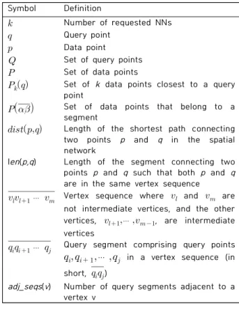
The symbols and notations used in this study are listed in Table 1. To simplify the presentation, we denote __{  }⋯ _ by __, where query points

__{  }⋯ _ are located in the same vertex sequence.

Symbol Definition

 Number of requested NNs

 Query point

 Data point

 Set of query points

 Set of data points

_ Set of k data points closest to a query point

^ Set of data points that belong to a segment

 Length of the shortest path connecting two points p and q in the spatial network

len(p,q) Length of the segment connecting two points p and q such that both p and q are in the same vertex sequence

__⋯ _ Vertex sequence where _ and _ are not intermediate vertices, and the other vertices, ⋯_{ }, are intermediate vertices

__{ }⋯ _ Query segment comprising query points

_ _{  }⋯ _ in a vertex sequence (in short, __)

adj_seqs(v) Number of query segments adjacent to a vertex v

Table 1. Definitions of symbols

III. The Proposed Scheme

1. Grouping adjacent query points

In this section, we consider an MkNN query in a spatial network, as shown in Figure 2. For

 ^___, and  ^____^{, we} consider a kNN query that retrieves data points closest to each query point q in Q. For simplicity, we assume that q1, q2, q3, and q4 request one, two, one, and two data points closest to them, respectively, which means that _ _  and

_ _ .

Algorithm 1: BANK()

Input: : set of query points, : set of data points

Output: : set of ordered pairs of each query point q in Q and its kNN set, i.e., 〈^〉∣∈^.

1 ← ∅ // the result set  is initialized to the empty set.

2 // adjacent query points in the same vertex sequence are grouped into a query group, which is explained in Section III.1.

3 ←group_points() // adjacent query points __{  }⋯_ in a vertex sequence are grouped into __. 4 // data points closest to each query point in __ are retrieved, which is detailed in Algorithm 2.

5 for each query segment __∈ do

6 ^__←BkNN_search^__ // ^__^〈^〉^{∣∈}_

7 ←∪^_ // the result for each query point in a query group __ is added to . 8 return  // is returned after the BkNN search for all query groups in is executed.

(a) Distribution of query and data points at _

(b) Distribution of query and data points at _ Fig. 2. Population of query and data points at

timestamps _ and _

Figure 2 shows the population of the query and data points at timestamps _ and _. Here, we assume that both the query and data points move arbitrarily along the spatial network. In this section, we focus on evaluating MkNN queries at timestamp, _, in Figure 2(a).

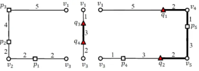
Fig. 3. Grouping of adjacent query points into query segments

Figure 3 illustrates a sample grouping of adjacent query points. Two query points, q1and q2,

in a vertex sequence, ____, are transformed into a query segment, __, and the other two query points, q3and q4, in a vertex sequence, __, are grouped into another query segment, __. Therefore, a set of query points,  ^__ _ can be transformed into a set of query groups,

^__ __.

2. BANK algorithm

Algorithm 1 describes the BANK algorithm for the MkNN search over spatial networks. The result set Π is initialized to an empty set (line 1). In the first step (lines 2―3), adjacent query points

__{  }⋯  _ in the same vertex sequence are grouped into a query segment __. Therefore, a set Q of query points is converted into a set  of query groups. The batch kNN (BkNN) search for a query segment __ is performed to obtain data points closest to each query point in __ (line 6).

Result Π^_ for __ is added to the query result Π^, where Π^_^〈^〉^{∈}_ ^(line

7). Subsequently, the query result Πis returned after performing the BkNN search for all query groups in  (line 8).

Algorithm 2 describes the BkNN search algorithm.

The BkNN search groups query points and batch execution to avoid redundant network traversal. This algorithm comprises two steps. First, two kNN queries are issued for the query segment __. We carefully determined the location of kNN queries

Algorithm 2: BkNN_search^__

Input: __: query segment, : set of data points

Output: ^_: set of ordered pairs of each query point q in __ and its kNN set, i.e., ^_^〈^〉∣∈__^.

1 ^__← ∅ // ^__ is initialized to an empty set

2 // assume that a query segment __ belongs to a vertex sequence __ and that _ (_) is closer to _ (_) than _ (_).

3 // step 1: a set of candidate data points is computed for all query points in __. 4 if adj_seqs^^{≥ and adj_seqs}^^{≥ then}

5 _

←max^_{  }⋯_ ^{// }is the max kvalue of __{  }⋯_ in query segments adjacent to _.

6 _

_^^←kNN_query^_ ^{// k}NN query is evaluated for _ and its kNN set is saved to _

_^^.

7 _

← max^_{  }⋯_ ^{// }_is the max k value of __{  }_⋯_ in query segments adjacent to _.

8 _

_^^←kNN_query^_ ^{// k}NN query is evaluated for _ and its kNN set is saved to _

_^^.

9 _{ ←}_

^^∪_

^^∪^__ // _ is the set of candidate data points for __. 10 else if adj_seqs^^{≥  and adj_seqs}^^{ then}

11 _

←max^_{  }⋯_ ^{// }is the max kvalue of __{  }⋯_ in query segments adjacent to _.

12 _

_^^←kNN_query^_ ^{// k}NN query is evaluated for _ and its kNN set is saved to _

_^^.

13 _

← max^_{  }⋯_ // _is the max k value of query points __{  }⋯_ in __.

14 _

_^^←kNN_query^_ ^{// k}NN query is evaluated for _ and its kNN set is saved to _

_^^.

15 _{ ←}_

_^^∪_^^∪^_ // _ is the set of candidate data points for __. 16 else if adj_seqs^^{ and adj_seqs}^^{≥ then}

17 _

←max^_{  }⋯_ // _

is the max kvalue of query points __{  }⋯_ in __.

18 _

_^^←kNN_query^_ ^{// k}NN query is evaluated for _ and its kNN set is saved to _

_^^.

19 _

← max^_{  }_⋯_ ^{// }is the max k value of __{  }⋯_ in query segments adjacent to _.

20 _

_^^←   ^_ ^{// k}NN query is evaluated for _ and its kNN set is saved to _

_^^.

21 _{ ←}_

_^^∪_



^^∪^_ // _ is the set of candidate data points for __. 22 else

23 _

←max^_{  }⋯_ // _

is the max kvalue of query points __{  }⋯_ in __.

24 _

_^^←kNN_query^_ ^{// k}NN query is evaluated for _ and its kNN set is saved to _

_^^.

25 _

←_

 // _

 is the same value as _

.

26 _

_^^←kNN_query^_ ^{// k}NN query is evaluated for _ and its kNN set is saved to _

_^^.

27 _{ ←}_

_^^∪_^^∪^_ // _ is the set of candidate data points for __.

28 // step 2: a set of kNNs for each query point in __ is computed using the set _ of candidate data points.

29 for each query point ∈__ do

30 // kNN search for a query point qis performed using a set _ of candidate data points for __.

31 _←kNN_search^{} ^{// k}NN search for qis performed using a set _ of candidate data points.

32 ^_^←^_^∪ 〈^〉 ^{// the} kNN set for qis saved to _, which is added to ^_^.

33 return // query result ^_ is returned for __.

using the number of query segments adjacent to an intersection vertex _ (_) in __ to share the results of kNN queries among the query segments adjacent to an intersection vertex. We assume that

__ belongs to __ and that _(_) is closer to _ (_) than _ (_). The location of one kNN query is either

_ or _, and the location of another kNN query is either _ or _. If more than two query segments are

adjacent to _, i.e., adj_segs^^{≥ , } issues a kNN query with _

 max^ _{  }⋯ _assuming that

__{  }⋯ _ belong to query segments adjacent to

_ and __{  }⋯  _ have __{  }⋯  _, respectively; otherwise, _ issues a kNN query with

_ max^_{  }⋯ _ ^{assuming that}

__{  }⋯  _ constitute __ and _ _{  }⋯  _ have

__{  }⋯_, respectively. Similarly, if more than