Evaluation and Predicting PM₁₀ Concentration Using Multiple Linear Regression and Machine Learning

https://doi.org/10.7780/kjrs.2020.36.6.3.7 ISSN 2287-9307 (Online)

Article

다중선형회귀와 기계학습 모델을 이용한 PM

10

손상훈 ¹⁾·김진수 ^2)†

Evaluation and Predicting PM

Concentration Using Multiple Linear Regression and Machine Learning

Sanghun Son

· Jinsoo Kim

Abstract: Particulate matter (PM) that has been artificially generated during the recent of rapid industrialization and urbanization moves and disperses according to weather conditions, and adversely affects the human skin and respiratory systems. The purpose of this study is to predict the PM

concentration in Seoul using meteorological factors as input dataset for multiple linear regression (MLR), support vector machine (SVM), and random forest (RF) models, and compared and evaluated the performance of the models. First, the PM

concentration data obtained at 39 air quality monitoring sites (AQMS) in Seoul were divided into training and validation dataset (8:2 ratio). The nine meteorological factors (mean, maximum, and minimum temperature, precipitation, average and maximum wind speed, wind direction, yellow dust, and relative humidity), obtained by the automatic weather system (AWS), were composed to input dataset of models. The coefficients of determination (R

) between the observed PM

concentration and that predicted by the MLR, SVM, and RF models was 0.260, 0.772, and 0.793, respectively, and the RF model best predicted the PM

concentration. Among the AQMS used for model validation, Gwanak-gu and Gangnam-daero AQMS are relatively close to AWS, and the SVM and RF models were highly accurate according to the model validations. The Jongno-gu AQMS is relatively far from the AWS, but since PM

concentration for the two adjacent AQMS were used for model training, both models presented high accuracy. By contrast, Yongsan-gu AQMS was relatively far from AQMS and AWS, both models performed poorly.

Key Words: PM

concentration, Meteorological Variables, Multiple Linear Regression, Support Vector Machine, Random Forest

요약 : 최근 급속한 산업화와 도시화로 인해 인위적으로 발생하는 미세먼지 (Particulate matter, PM)는 기상 조건 에 따라 이동 및 분산되면서 피부와 호흡기 등 인체에 악영향을 미친다 . 본 연구는 기상인자를 multiple linear Received December 14, 2020; Revised December 16, 2020; Accepted December 18, 2020; Published online December 23, 2020

1)

부경대학교 지구환경시스템과학부 공간정보시스템전공 박사과정생 (PhD Student, Division of Earth Environmental System Science (Major of Spatial Information Engineering), Pukyong National University)

2)

부경대학교 공간정보시스템공학과 부교수 (Associate Professor, Department of Spatial Information Engineering, Pukyong National University)

†

Corresponding Author: Jinsoo Kim ([email protected])

This is an Open-Access article distributed under the terms of the Creative Commons Attribution Non-Commercial License

(http://creativecommons.org/licenses/by-nc/3.0) which permits unrestricted non-commercial use, distribution, and reproduction in

any medium, provided the original work is properly cited.

1. 서론

급속한 산업화에 따른 인구증가 , 도시화, 화석 연료 소 비 증가로 야기된 대기 오염은 인체에 여러 질병들을 야 기시키며 인류가 해결해야 할 중요한 문제 중 하나로 인 식되고 있다(Choubinet al., 2020; KampaandCastanas, 2008;

Saeed et al., 2017). 세계보건 기구(world health organization, WHO)는 2018년 한 해 동안 대기 오염 노출로 인해 세 계적으로 약 420만 명의 사망자가 발생했을 것으로 추 정하였다 (Stafoggia et al., 2019). 대기 오염은 4가지 그룹 ((a) SO

, NO

, CO 등과 같은 가스상 물질, (b) 다이옥신 과 같은 잔류성 유기오염물질 , (c) 납, 수은과 같은 중 금속 , (d) 미세먼지(particulate matter, PM))으로 분류하 고 있으며 (Kampa and Castanas, 2008), 그 중 PM는 자연 및 인위적 활동에 의해 생성되어 대기에 부유하는 혼합 물로써 그 크기와 구성이 다양한 대표적인 대기 오염 물 질 유형이다 . PM는 입자의 크기에 따라 PM

과 PM

등 으로 정의되며 , Global Burden of Disease(GBD)에 따르 면 PM은 인체 건강을 해치는 84개 위험 요소 중 6번째 주요 사망원인으로 지목되고 있다 (Saeed et al., 2017;

Stafoggia et al., 2019). 특히 자연적 배출원인 황사와 인위 적 배출원인 산업시설, 자동차 등으로부터 배출되는 PM

은 피부질환, 호흡기 및 심혈관계 질환 등 인체에 악영향을 미치며 , 산성비 등을 야기하여 생태계를 오염 시킬 뿐 아니라 지구 복사 수지에도 영향을 미친다 (Han et al., 2008).

지금까지 PM 농도 예측 모델링과 모니터링을 위한 다양한 노력이 이루어졌다 . 먼저 입력자료를 기상인자

만을 적용하여 전통적인 다중선형회귀(multiple linear regression, MLR)로 시간대별 그리고 일별 PM

농도를 예측하기 위한 시도와 함께 기상인자와 화학인자 또는 기상인자와 위성기반 AOD(aerosol optical depth) 자료 를 동시에 고려한 연구가 수행되었다 (Abdullah et al., 2020; Diaz-Robles et al., 2008; Munir, 2016; Özdemir and Taner, 2014; Slini et al., 2006; UI-Saufie et al., 2011; Zaman et al., 2017). 최근 PM

농도 예측을 위해 기상인자 및 기 상인자와 화학인자를 기계학습에 적용한 시도가 활발 히 이루어지고 있다(Arampongsanuwat and Meesad, 2012;

Ibrir et al., 2020; Ivanov et al., 2018; Li et al., 2017; Lim, 2019;

Mallet, 2020; Weizhen et al., 2014), 특히 Stafoggia et al.

(2019)와 Choubin et al. (2020)은 이상의 인자들과 함께 AOD, NDVI(normalized difference vegetation index), TWI (topographic wetness index), TRI(terrain ruggedness index) 등과 같은 인자를 고려한 시간대별 PM

농도를 예측하 고 그 결과를 보고하였다. 이상의 연구와 같이 다중선 형회귀와 기계학습 모델 바탕을 PM

농도 예측을 하 였으나 , 다중선형회귀와 기계학습 모델을 비교 평가한 연구는 미미했다 . 국립환경과학원은 기상상태에 따른 2차 미세먼지의 생성 등이 수도권 고농도 미세먼지 발 생에 크게 영향을 미치는 것을 밝힌 바 있다 (Lee, 2016).

따라서 본 연구는 고농도 미세먼지 발생이 빈번한 서울 시를 대상으로 기상인자를 바탕으로 통계기법과 기계 학습을 이용한 PM

농도 예측 모델링을 수행하고, 각 모델 간의 성능을 비교 및 평가하는데 그 목적을 둔다 . regression(MLR), support vector machine(SVM), 그리고 random forest(RF) 모델의 입력자료로 하여 서울시 PM

농도를 예측하고, 모델 간 성능을 비교 평가하는데 그 목적을 둔다. 먼저 서울시에 소재한 39개소 대기오염측

정망 (air quality monitoring sites, AQMS)에서 관측된 PM

농도 자료를 8:2 비율로 구분하여 모델 훈련과 검증 데

이터셋으로 사용되었다 . 또한 기상관측소(automatic weather system, AWS)에서 관측되고 있는 자료 중 9개 기상

인자 (평균기온, 최고기온, 최저기온, 일 강수량, 평균풍속, 최대순간풍속, 최대순간풍속풍향, 황사발생유무, 상

대습도)가 모델의 입력자료로 선정되었다. 각 AQMS에서 관측된 PM

농도와 MLR, SVM, 그리고 RF 모델에 의

해 예측된 PM

농도 간 결정계수 (R

)는 각각 0.260, 0.772, 그리고 0.793이었고, RF 모델이 PM

농도 예측에 가장

높은 성능을 나타냈다 . 특히 모델 검증에 사용되는 AQMS 중 관악구와 강남대로 AQMS는 상대적으로 AWS에

가까워 SVM과 RF 모델에서 높은 정확도를 나타냈다. 종로구 AQMS는 AWS에서 비교적 멀리 떨어져 있지만,

인접한 두 AQMS 데이터가 모델 학습에 사용되었기 때문에 두 모델에서 높은 정확도를 나타냈다. 반면 용산구

AQMS는 AQMS 및 AWS에서 비교적 멀리 떨어져 있기에 두 모델의 성능이 낮게 나타냈다.

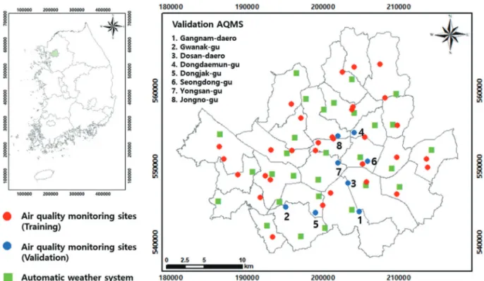
2. 연구대상지역

본 연구에서 매년 고농도 미세먼지가 빈번히 발생하 는 서울시를 연구대상지역으로 선정하였고 , 본 연구대 상지역 내에 39개소대기오염측정망(airqualitymonitoring sites, AQMS)과 29개소 방재기상관측소(automatic weather system, AWS)가 소재하고 있다(Fig. 1). 에어코리아는 2001년부터 AQMS에서 관측된 6가지 대기오염도물질 (PM

, PM

, O

, NO

, CO, SO

) 자료를 시간대별로 제 공하고 있으며 , 기상청은 1997년부터 방재기상관측을 통해 7가지 기상자료(기온, 풍향, 풍속, 강수량, 습도, 현 지기압 , 해면 기압)를 시간대별로 제공하고 있다. 서울 시 PM

농도는 2003년 이후 황사일을 제외하였을 때 감소 추이를 보이나 2012년 이후 오히려 증가는 추세 이고 , 환경부에서 제공하는 서울시 미세먼지 주의보 발 령 일수는 2013년에 2일에 불과했으나 2017년에 10일로 13년에 비해 5배 증가하였다(Hwang and Han, 2018; Kim and Kim, 2011). 따라서 2017년 1년 동안 관측된 AQMS 와 AWS 자료를 바탕으로 PM

농도 예측 성능을 평가 하였다 .

3. 방법론

1) 데이터셋

본 연구에서 PM

농도를 예측하기 위한 모델 내 입 력자료로는 AQMS에서 관측된 시간대별 PM

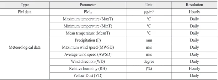
농도 자료와 기상청에서 제공하는 8개 일별 기상인자(평균 기온, 최고기온, 최저기온, 일 강수량, 평균풍속, 최대순 간풍속, 최대순간풍속풍향, 황사발생유무) 및 시간대 별 상대습도를 선정하였다 . PM

농도 자료는 특정 시 간대에 미관측된 자료에 의한 오차를 최소화하기 위해 일평균 PM

으로 합성하였다 . 기상인자 중 상대습도 는 일평균으로 재합성하였다 (Table 1). AQMS와 AWS 는 공간적으로 일치하지 않기 때문에 PM

농도는 각 AQMS에서 최단 거리에 위치한 AWS의 기상인자들을

매칭하였으며 , 황사발생유무는 기상청에서 제공하는

관측소별, 일별 자료를 취합하여 PM

일별 농도 데이 터와 매칭하였다. 이상의 결과로 39개 AQMS에서 구축 된 일별 데이터 셋은 총 13,969개이며, MLR 모델에서는 PM

농도를 종속변수로 , 매칭된 기상인자를 독립변수 로 사용하였다 . Support vector machine(SVM)과 random forest(RF) 모델의 경우 39개 AQMS 중 약 80%에 해당하 는 31개 AQMS에서의 11,096개 자료가 훈련을 위해 사

Fig. 1. The specifications of study area.

용되었고 , 나머지 8개 AQMS 자료인 2,873개 자료가 검 증을 위한 데이터셋으로 선정되었다 .

2) MLR

MLR 모델은 종속변수와 여러 독립변수 간의 관계를 선형 방정식을 이용하여 변수 간의 관계를 모델링하는 기법이며 , MLR 방정식은 식 (1)과 같다. PM

농도 예측 을 위한 종속변수는 PM

농도이며 , 독립변수는 PM

인자를 제외한 기상인자들이다 .

Y = α

+ α

X

+ α

X

+ … + α

X

+ ε (1) 여기서 Y는 종속변수를 의미하며, α

는 상수계수 , α

, α

, …, α

와 X

, X

, …, X

는 각각 회귀계수와 독립변수, 그리고 ε는 확률 오차를 의미한다.

3) SVM

SVM은 기계학습 중 하나로 데이터 분석 및 패턴 인식, 자료 분석 등을 위한 지도학습 모델로 여러 분야에서 그 정확도가 높은 것으로 보고되고 있다 . SVM 모델은 SRM(structural risk minimization)에 기반으로 전체 집단 을 세분화하여 각 집단에 대한 경험적 오류를 최소화 하는 의사결정함수를 사용하기 때문에 일반화가 용이 하며 , 다양한 커널을 이용하여 선형 데이터뿐만 아니라 비선형 데이터에 대한 분석도 가능하다는 장점이 있다 (Cortes and Vapnik, 1995).

PM

농도 예측을 위해 4개 커널 중 비교적 높은 정확 도를 나타내는 것으로 보고된 바 있는RadialBasisFunction (RBF) 커널이 선정되었다(Pourghasemi et al., 2018). RBF

커널의 파라미터들은 학습 오류의 최소화와 모델의 복 잡성 사이의 값을 나타내는 Cost(C)와 일부 고차원 특성 공간으로의 비선형 매핑을 정의하는 gamma가 있다 (Chen et al., 2011). SVM 모델은 R의 ‘e1071’ 패키지를 이 용하여 RBF 모델을 구축하였으며, 최적의 RBF 모델 구 축을 위해 grid-search 기법을 이용하여 주요 파라미터 C 와 gamma에 대한 하이퍼 파라미터를 결정하였다.

4) RF

RF 모델은 앙상블 기법을 사용하는 다수의 의사결정 나무 (decision tree, DT)로 구성된 기계학습이다. 이것은 다소 데이터에 대한 의존도가 높고 비교적 낮은 정확도 를 나타내는 DT의 단점을 보완하기 위해 bagging과 bootstrap 기법을 결합한 모델이다. 또한 RF는 신경망과 같은 전통적인 기계학습과 달리 데이터 양이 방대하더 라도 처리속도가 빠르며 , 변수 간의 비선형성을 잘 반 영하는 모델이다 . 그러나 독립변수들을 랜덤으로 추출 하기 때문에 결과에 대한 해석이 어렵다는 단점이 있다 (Breiman, 2001).

RF는 트리 수를 나타내는 ntree와 전체 데이터에 대 한 선택된 변수의 수인 mtry의 파라미터들이 있으며 (Liu et al., 2019), 본 연구에서 RF 모델은 R의 ‘Random Forest’와 ‘Caret’ 패키지를 이용하여 구축되었고, 최적의 모델 구축을 위해 grid-search 기법을 이용하여 ntree와 mtry에 대한 하이퍼 파라미터를 결정하였다.

Table 1. Summary of the input dataset to predict PM

concentration in this study

Type Parameter Unit Resolution

PM data PM

μg/m

Hourly

Meteorological data

Maximum temperature (MaxT) °C Daily

Minimum temperature (MinT) °C Daily

Mean temperature (MeanT) °C Daily

Precipitation (P) mm Daily

Maximum wind speed (MWSD) m/s Daily

Average wind speed (AWSD) m/s Daily

Wind direction (WD) degree Daily

Relative humidity (RH) (%) Hourly

Yellow Dust (YD) Daily

4. 결과 및 토의

1) MLR

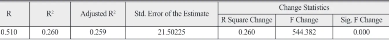
SPSS version 25를 이용하여 MLR을 수행한 결과, 상 관계수는 0.510, 결정계수(R

)는 0.260, 수정된 R

는 0.259 로 모델의 정확도는 높지 않으나 모형의 유의 수준을 나 타내는 Significant F의 값이 0.000으로 나타나 유의한 통 계모형으로 설명될 수 있다(Table 2).

PM

농도 예측을 위해 산출된 회귀식은 식 (2)와 같다.

Table 3은 각 인자 별 계수 값과 독립변수들의 상대적 중요도 결과를 나타낸 것으로 황사발생유무가 PM

농 도에 가장 많은 영향을 미치는 것으로 나타났으며 평균 풍속, 최고기온, 최저기온 순으로 영향을 미치는 것으 로 나타났다. 유의확률 Sig.가 0.05 이하일 때 독립변수 가 종속변수에 유의한 영향을 미치는 것을 의미하며 , 최 소기온을 제외한 변수들은 PM

농도 예측에 유의미한 변수로 설명되었다 .

PM

= 36.993 – 2.258 * MaxT – 0.193 * MinT + 1.985 * MeanT – 0.167 * P + 0.377 * MWSD – 3.313 *AWSD + 0.025 * WD + 0.030 * RH + 51.816 * YD (2)

2) SVM

RBF 커널의 하이퍼 파라미터를 추정하기 위해 C는 7개(0.001, 0.01, 0.1, 1, 10, 100, 1000)를, gamma는 9개 (0.001, 0.01, 0.1, 1, 2, 3, 4, 5, 10)를 적용하였다. grid-search 기법을 통해 최종적으로 결정된 최적 C와 gamma는 각 각 10과 3으로 선정되었다. 하이퍼 파라미터를 적용한 모델의 훈련과 검증 정확도 R

은 각각 0.922와 0.772로 나타났다 (Fig. 2).

3) RF

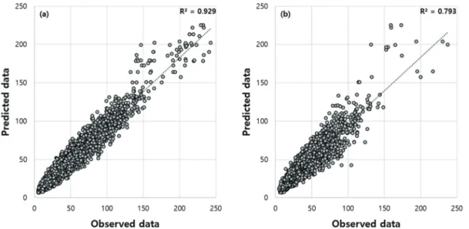
RF의 하이퍼 파라미터를 추정하기 위해 mtry 는 3, 4, 5, 6으로, ntree 는 100부터 5000까지 100단위로 나누어 적용하였다 . grid-search 기법을 통해 최종적으로 결정된 최적 mtry와 ntree는 각각 6과 300으로 선정되었다. 하이 퍼 파라미터를 적용한 모델의 훈련과 검증 정확도 R

는 각각 0.929과 0.793로 나타났다(Fig. 3).

RF 모델은 feature selection의 두 인자 % IncMSE와 IncNodePurity를 사용하여 모델에 영향을 주는 인자의 중요도를 판별할 수 있다 . % IncMSE는 해당 인자를 모 형에서 제외했을 때 예측 오류인 MSE(mean square error) 의 증가 추정치를 나타내는 것으로 식 (3)에 의해 산출 되며 , % IncMSE 값이 높을수록 모델에 영향을 많이 주 Table 2. Model summary of multiple linear regression analysis

R R

Adjusted R

Std. Error of the Estimate Change Statistics

R Square Change F Change Sig. F Change

0.510 0.260 0.259 21.50225 0.260 544.382 0.000

Table 3. Coefficients of independent variables Unstandardized Coefficients Standardized Coefficients

t Sig.

B Std. Error Beta

(constant) 36.993 1.541 24.007 0.000

MaxT -2.258 0.336 -0.953 -6.717 0.000

MinT -0.193 0.180 -0.083 -1.073 0.283

MeanT 1.985 0.181 0.859 10.960 0.000

P -0.167 0.014 -0.095 -11.705 0.000

MWSD 0.377 0.121 0.038 3.116 0.002

AWSD -3.313 0.408 -0.103 -8.125 0.000

WD 0.025 0.002 0.097 12.831 0.000

RH 0.030 0.015 0.019 1.989 0.047

YD 51.816 0.963 0.399 53.804 0.000

는 인자이다 (Seo, 2016).

% IncMSE = * 100 (3) IncNodePurity는 Gini index를 이용하여 각 인자들의 노드 불순도 (node impurity)에 대한 개선 기여도를 나타 낸 것이며 , 그 값이 클수록 모델 성능에 더 중요한 인자 이다 . 본 연구에서 상대습도와 황사발생유무가 PM

농 도 예측 성능에 크게 기여하는 반면 , 최고 기온와 평균 풍속은 상대적으로 기여도가 낮은 것으로 나타났다 (Fig. 4).

이상과 같이 SVM과 RF 모델이 MLR 모델에 비해 서울시 PM

농도 예측에서 매우 높은 정확도를 나타 냈다. 이러한 결과는 기상인자를 이용하여 PM

농도를 예측한 선행연구에서 비선형과 앙상블 모델이 다중선 형회귀에 비해 그 성능이 높다고 보고된 것과 동일하다 (Diaz-Robles et al., 2008; Özdemir and Taner, 2014). 본 연 구에서 제시된 SVM 모델의 예측 성능(R

=0.772)은 Ibrir et al. (2020)에 의해 보고된 결과(R

=0.780)와 거의 유사 하며 , RF 모델을 이용한 예측 성능은 기존 선행연구 결 과에 비해 매우 우수하게 나타났다 (Bozdag˘ et al., 2020;

MSE(n) – MSE(0) MSE(0)

Fig. 2. The scatter diagrams in SVM: (a) trained PM

concentration,(b) predicted PM

concentration.

Fig. 3. The scatter diagrams in RF: (a) trained PM

concentration,(b) predicted PM

concentration.

Grange et al., 2018; Mallet, 2020).

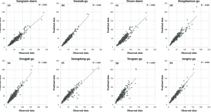
모델 검증에 사용된 8개 AQMS 중 관악구, 강남대로, 그리고 종로구에서 SVM과 RF 모델의 R

이 0.904-0.948

로 높게 나타났다 . 이는 관악구와 강남대로 AQMS에서

인접한 위치에 AWS가 소재하고 있는 점과 종로구

AQMS와 비교적 인접한 2개 AQMS 자료가 모델 학습

Fig. 5. The scatter diagrams of each validation AQMS in SVM.

Fig. 4. The important measure for each variable according to %IncMSE and IncNodePurity.

에 사용되었기 때문인 것으로 판단된다 . 반면 모델 학 습에 사용된 AQMS 뿐만 아니라 AWS와 상대적으로 먼 거리에 위치한 용산구 AQMS에서 두 모델의 R

이 0.806- 0.826으로 비교적 낮게 나타났다(Fig. 5, Fig. 6).

5. 결론

본 연구는 에어코리아에서 제공하는 PM

농도와 PM

농도에 영향을 미치는 기상인자를 바탕으로 MLR, SVM, 그리고 RF 모델을 이용하여 서울시 PM

농도를 예측하고 , 그 성능을 평가하였다. 3가지 모델의 훈련과 검증을 단계적으로 수행한 결과 , 앙상블 모델인 RF의 예측 성능이 가장 높게 나타났으며 , 다음으로 SVM과 MLR 순으로 나타났다. 본 연구에서 사용된 9개 기상인 자 중 상대습도와 황사발생유무가 RF 모델의 예측 성 능에 가장 크게 기여하였고 , 최고 기온와 평균 풍속은 상대적으로 낮은 기여도를 나타냈다. 또한 관악구, 강남 대로, 종로구와 같이 인접한 위치에 AWS 또는 모델 학 습을 위한 AQMS가 소재하는 경우 SVM과 RF 모델의 예측 정확도가 높고 , 반대의 경우인 용산구에서 두 모 델의 정확도가 가장 낮은 점에 비춰볼 때 , AQMS와 AWS 간 인접성과 훈련 데이터 셋의 공간적 분포는

PM

농도 예측에 매우 큰 영향을 미치는 것으로 판단 된다. 또한 PM

농도에 유의미하게 영향을 미치는 AOD, NDVI, 토지피복 등을 고려한 다양한 시도를 통 해 PM

농도 예측의 정확도가 보다 향상될 수 있을 것 으로 기대된다 .

사사

이 논문은 부경대학교 자율창의학술연구비 (2019년) 에 의하여 연구되었음 .

References

Abdullah, S., N. N. L. M. Napi, A. N. Ahmed, W. N. W.

Mansor, A. A. Mansor, M. Ismail, A. M. Abdullah, and Z. T. A. Ramly, 2020. Development of Multiple Linear Regression for Particulate Matter(PM

) Forecasting during Episodic Transboundary Haze Event in Malaysia, Atmosphere, 11(289): 1-14.

Arampongsanuwat, S. and P. Meesad, 2012. PM

Prediction Model by Support Vector Regression

Fig. 6. The scatter diagrams of each validation AQMS in RF.

Based on Particle Swarm Optimization, Advanced Materials Research, 403-408: 3693-3698.

Bozdag˘, A., Y. Dokuz, and Ö. B. Gökçek, 2020. Spatial prediction of PM

concentration using machine learning algorithms in Ankara, Turkey, Environmental Pollution, 263(A): 1-10.

Breiman, L., 2001. Random Forest, Machine Learning, 45(1): 5-32.

Chen, H. L., B. Yang, J. Liu, and D. Y. Liu, 2011. A support vector machine classifier with rough set- based feature selection for breast cancer diagnosis, Expert Systems with Applications, 38(7): 9014- 9022.

Choubin, B., M. Abdolshahnejad, E. Moradi, X. Querol, A. Mosavi, S. Shamshirband, and P. Ghamisi, 2020. Spatial hazard assessment of the PM

using machine learning models in Barcelona, Spain, Science of The Total Environment, 701(20):

1-11.

Cortes, C. and V. Vapnik, 1995. Support-vector networks, Machine Learning, 20: 273-297.

Diaz-Robles, J. A., J. C. Ortega, J. S. Fu, G. D. Reed, J. C. Chow, J. G. Watson, and J. A. Moncada- Herrera, 2008. A hybrid ARIMA and artificial neural networks model to forecast particulate matter in urban areas: The case of Temuco, Chile, Atmospheric Environment, 42(35): 8331-8340.

Grange, S. K., D. C. Carslaw, A. Lewis, E. Boleti, and C. Heuglin, 2018. Random forest meteorological normalisation models for Swiss PM

trend analysis, Atmospheric Chemistry and Physics Discussions, 18(9): 6223-6239.

Han, J. H., M. H. Lee, and Y. S. Ghim, 2008. Cluster Analysis of PM

Concentrations from Urban Air Monitoring Network in Korea during 2000 to 2005, Journal of Korean Society for Atmospheric Environment, 24(3): 300-309 (in Korean with English Abstract).

Hwang, I. C. and J. S. Han, 2018. A Feasibility Study of a New Urban Access Regulation in Seoul:

Policy Design, Public Acceptance, and the Expected Effects, The Seoul Institute, Seoul, KOR.

Ibrir, A., Y. Kerchich, N. Hadidi, H. Merabet, and M.

Hentabli, 2020. Prediction of the concentrations of PM1, PM

, PM

, and PM

by using the hybrid dragonfly-SVM algorithm, Air Quality, Atmosphere

& Health, 2020: 1-11.

Ivanov, A., D. Voynikova, M. Stoimenova, S. Gocheva- Ilieva, and I. Iliev, 2020. Random Forests Models of Particulate Matter PM

: A Case Study, Proc. of 2018 American Institute of Physics Conference Proceedings, Albena, BUL, Jun. 20-25, vol. 2025 p. 03001.

Kampa, M. and E. Castanas, 2008. Human health effects of air pollution, Environmental Pollution, 151(2):

362-367.

Kim, W. S. and J.A. Kim, 2011. A Study of Building Customized Management Strategies Based on Local PM

Emission, The Seoul Institute, Seoul, KOR.

Kirasich, T., T. Smith, and B. Sadler, 2018. Random Forest vs Logistic Regression: Binary Classification for Heterogeneous Datasets, SMU Data Science Review, 1(3): 1-24.

Lee, M. H., 2016. Korea-China collaborative study to abate trans-boundary air pollution(II), National Institute of Environmental Research, Research Report, Incheon, KOR.

Li, Y. and Y. Tao, 2017. PM

Concentration Forecast Based on Wavelet Support Vector Machine, Proc.

of 2017 International Conference on Sensing, Diagnostics, Prognostics, and Control, Shanghai, CHA, Aug. 16-18, pp. 383-386.

Lim, J. M., 2019. An Estimation Model of Fine Dust Concentration Using Meteorological Environment Data and Machine Learning, Journal of Information Technology Services, 18(1): 173-186 (in Korean with English Abstract).

Liu, K., D. Tian, H. Xu, H. Wang, and G. Yang,

2019. Quantitative analysis of toxic elements in

polypropylene (PP) via laser-induced breakdown spectroscopy (LIBS) coupled with random forest regression based on variable importance (VI- RFR), Analytical Methods, 11: 4769-4774.

Mallet, M.D., 2020. Meteorological normalisation of PM

using machine learning reveals distinct increases of nearby source emissions in the Australian mining town of Moranbah, Atmospheric pollution research, 2020: 1-16.

Munir S., 2016. Modelling the non-linear association of particulate matter(PM

) with meteorological parameters and other air pollutants-a case study in Makkah, Arabian Journal of Geosciences, 9(64): 1-13.

Özdemir, U. and S. Taner, 2014. Impacts of Meteorological Factors on PM

: Artificial Neural Networks(ANN) and Multiple Linear Regression(MLR) Approaches, Environmental Forensics, 15(4): 329-336.

Pourghasemi H. R., A. G. Jirandeh, B. Pradhan, C. Xu, and C. Gokceoglu, 2018. Landslide susceptibility mapping using support vector machine and GIS at the Golestan Province, Iran, Journal of Earth System Science, 122(2): 349-369.

Saeed, S., L. Hussain, I. A. Awan, and A. Idris, 2017.

Comparative Analysis of different Statistical Methods for Prediction of PM

and PM

Concentrations in Advance for Several Hours, International Journal of Computer Science and Network Security, 17(11): 45-52.

Seo, J. D., 2016. Foreign Exchange Rate Forecasting Using the GARCH extended Random Forest Model, Journal of Industrial Economics and Business, 29(5): 1607-1628 (in Korean with

English abstrsct).

Slini, T., A. Kaprara, K. Karatzas, and N. Moussiopoulos, 2006. PM

forecasting for Thessaloniki, Greece, Environmental Modelling & Software, 21(4):

559-565.

Stafoggia, M., T. Bellander, S. Bucci, M. Davoli, K. de Hoogh, F. de’ Donato, C. Gariazzo, A. Lyapustin, P. Michelozzi, M. Renzi, M. Scortichini, A. Shtein, G. Viegi, I. Kloog, and J. Schwartz, 2019. Estimation of daily PM

and PM

concentrations in Italy, 2013-2015, using a spatiotemporal land-use random-forest model, Environment International, 124: 170-179.

UI-Saufie, A., A. Yahya, N. Ramli, and H. Hamid, 2011. Comparison Between Multiple Linear Regression And Feed forward Back propagation Neural Network Models For Predicting PM

Concentration Level Based On Gaseous And Meteorological Parameters, International Journal of Applied Science and Technology, 1(4): 42-49.

Weizhen, H., L. Zhengqiang, Z. Yuhuan, X. Hua, Z.

Ying, L. Kaitao, L. Donghui, W. Peng, and M.

Yan, 2014. Using support vector regression to predict PM

and PM

, IOP Conference Series:

Earth and Environmental Science, Proc. of 2013 35th International Symposium on Remote Sensing of Environment (ISRSE35), Beijing, CHN, Apr.

22-26, vol.17, pp. 012268.1-012268.6.

Zaman, N. A. F. K., K. D. Kanniah, and D. G.

Kaskaoutis, 2017. Estimating Particulate Matter

using satellite based aerosol optical depth and

meteorological variables in Malaysia, Atmospheric

Research, 193: 142-162.