The study of the calculation of energy consumption load for heating and cooling in building using the Laplace Transform solution

Introduction

Reducing energy consumption load in residential and in- dustrial buildings has been focused for a long time due to rapidly rising costs of heating in winter and cooling in sum- mer time, About more than 10% of the total energy in Korea is required for residential space heating and cooling. Some works (Peavy et al., 1973, Kusuda, 1976) have been done and many methods have been developed to obtain energy consumption loads for residential buildings. This concept is first introduced using what they call room thermal response factors (Stephenson and Mitalas, 1967, Mitalas and Stephen- son, 1967). Their method for procedure is that the internal wall surface temperatures of residential buildings and cool- ing or heating load are first calculated in a rigorous manner for several typical constructions. A computer model for sim- ulating heat flow by conduction through walls and roofs is developed based on the transmission matrix method (Buff-

ington, 1975). The transmission matrix method relates the periodic temperature and heat flux on one side of a homoge- neous layer to the periodic temperature and heat flux on the other side by means of a transmission matrix. The main ad- vantage of the transmission matrix method is the simplicity with which the model describes transient inside air temper- atures.

Gadgil et al. (1982) find that variation in convection coef- ficients can have substantial effects on thermal loads for a structure. Computer programs are developed to simulate nu- merically natural convection in two and three dimensional room geometries. Christensen and Perkins (1981) describe the effects of typical internal gain assumptions in energy cal- culations. The results of this study indicate that calculations of annual heating and cooling loads are sensitive to the av- erage internal gains, but, in most cases, are relatively insen- sitive to hourly variations in internal gains.

The study of the calculation of energy consumption load for heating and cooling in building using the Laplace Transform solution

Kyu-Il H

*

Department of Mechanical System Engineering, Pukyong National University, Busan 608-739, Korea

The Laplace Transform solution is used as a mathematical model to analyse the thermal performance of the building constructed using different wall materials. The solution obtained from Laplace Transform is an analytical solution of an one dimensional, linear, partial differential equation for wall temperature profiles and room air temperatures. The main purpose of the study is showing the detail of obtaining solution process of the Laplace Transform. This study is conducted using weather data from two different locations in Korea: Seoul, Busan for both winter and summer conditions. A comparison is made for the cases of an on- off controller and a proportional controller. The weather data are processed to yield hourly average monthly values. Energy con- sumption load is well calculated from the solution. The result shows that there is an effect of mass on the thermal performance of heavily constructed house in mild weather conditions such as Busan. Building using proportional control experience a higher comfort level in a comparison of building using on-off control.

Keywords : Laplace Transform, steady state, energy consumption load, thermal performance, comfort level

http://dx.doi.org/10.3796/KSFT.2014.50.3.292

*Corresponding author: [email protected], Tel: 82-51-629-6194, Fax: 82-51-629-6188

< Original Article>

Sodha et al. (1986) predict energy loads using an Admit- tance method and a Fourier method. The Admittance method is used to solve the problem using matrix equations, relating the temperature and energy cycle. the aim of the study is to compare the results obtained by two methods for the same system under identical conditions. It is shown that the two methods match well. The maximum deviation in the auxil- iary energy rate at any hour is about 100 of the amplitude.

Although there are sophisticated energy calculation pro- cedures available (Incropera et al., 2013) based upon the de- tailed dynamic simulation of hourly and sometimes minute-by-minute building performance inclusive of shell heat transfer, utility system, and equipment, the application of these detailed procedures requires large-scale computer systems, extensive labor to prepare input decks, and signifi- cant computer usage costs. Large computer programs are generally impractical for most applications. In other words, refined and sophisticated calculation procedures are unfor- tunately both time-consuming and expensive.

The main purpose of this study is showing how to obtain the Laplace transformation solution in detail as a mathemat- ical model. And the thermal performance of the building con- structed with different wall materials can be analysed using Laplace transform solution.

Theoretical formulation for analytical solution The formulation of an analytical method for obtaining wall temperature profile, room air temperature, and energy con- sumption load is presented. Two houses with different wall

materials in different weather conditions are modelled. Each test house is a 6.1m by 6.1m by 2.3m one-room house. The houses have identical floor plans and orientations, and are identical except for wall construction, which is as follows:

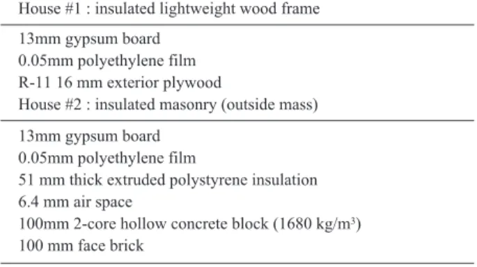
insulated lightweight wood frame; insulated masonry with outside mass. The details of the wall construction for each of the two houses are presented in Table 1.

Weather data for two cities (Seoul, Busan) are used in this study. Twenty-four discrete data points from weather data files are converted to continuous form via a Fast Fourier Transform (Brigham, 1974). Each house is modelled by a single homogeneous wall and an air node.

The thermal system is illustrated in Fig. 1. It is represented mathematically by two energy balances: one on the wall, and the other on the room air. The case studied represents a linear flow of heat in a solid wall bounded by a pair of parallel planes, at x〓0 and x〓L (Kreyszig, 2011). The system is considered as one-dimensional. the heat flow occurs princi- pally in the direction perpendicular to the thickness of the

Fig. 1. Thermal system.

House #1 : insulated lightweight wood frame 13mm gypsum board

0.05mm polyethylene film R-11 16 mm exterior plywood

House #2 : insulated masonry (outside mass) 13mm gypsum board

0.05mm polyethylene film

51 mm thick extruded polystyrene insulation 6.4 mm air space

100mm 2-core hollow concrete block (1680 kg/m³) 100 mm face brick

wall (x-direction).

Under this study there is no heat generation within the wall, and the energy balance, after some manipulation, yields:

∂

T/∂x

〓(1/a)∂T/∂t (1)

Two corresponding boundary conditions to the above lin- ear, second-order, partial differential equation are:

－k∂T/∂x (x〓0)〓âS* + h

(T

－T

) (2)

－k∂T/∂x (x〓L)〓－h

(T

－T

) (3)

The initial condition for the wall temperature is expressed in polynomial form as:

T (x, 0)〓 ∑

n〓0

a

x

(4)

The energy balance (Oosthuizen and Naylor, 1999) for the room air temperature including heat transfer from the inside surface of the wall, infiltration loss I, and auxiliary heat input Q, is:

C

dT

/dt 〓－h

A (T

－T

) －C

′I (T

－T

) + Q (5)

C

〓(rC

)

V

(6)

C

′〓(rC

)

V

(7)

I′〓CA

′I/C

(8)

The parameters, h

, h

, C

, C

′ and I are assumed constant.

The corresponding initial condition to equation (5) is as fol- lows:

T

(0)〓T

(9)

There exists a coupling between wall and room air tem- peratures (Modelst, 1993), and the two sets of equations must be solved simultaneously. Weather data for two cities are used in this study. weather data files are used to obtain hourly values of the solar flux and ambient temperature. The weather data input to the analytical model is finally repre- sented in the following form:

S* (t)〓b

+

∑

i〓1

[b

cos (w

t + F

) + c

sin (w

t + F

)] (10) T

(t)〓d

+

∑

i〓1

[d

cos (w

t + F

) + e

sin (w

t + F

)] (11) where b

is the DC component of the solar flux and d

is the DC component of the ambient temperature. Such analyt- ical functions can be easily integrated and differentiated so as to facilitate the solution process. The calculation method to obtain effective properties for buildings and thermal trans- port parameters such as heat transfer coefficients are intro- duced.

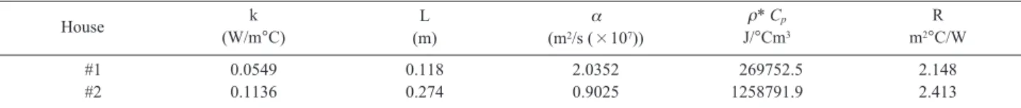
The effective properties based on Marks′ standard hand- book (1978) of a homogeneous wall, which represents the actual building ls wall, are necessary to obtain an analytical solution. Use of such properties is inevitable to simplify the analytical solution. The effective properties are shown in Table 2.

Effective thermal properties such as thermal conductivity, thermal diffusivity, thermal capacitance, and thermal resist- ance, which represent the wall as a single homogeneous unit can be computed based on matching: (1) the wall length (summation of the Length of wall components), (2) the ther- mal resistance, (3) the thermal capacitance of the materials comprising the wall, and additionally, (4) the time delays for a thermal pulse to penetrate the wall.

It is desired to maintain comfort inside the building. In order to accomplish this practically, the rate of supply of heat to the building is regulated by a controller. Two types of con- trol mechanisms are chosen for investigation. One is a simple

‘on-off ’controller; the other is a proportional controller.

The on-off controller is very popular both in residential and commercial buildings because of its simplicity of oper- ation (Winn, 1982). The control logic is depicted in Fig. 2.

The rate of supply of heat (Q) from the auxiliary energy source switches on or off depending on the difference be- tween the inside room air temperature and the set-point tem-

Table 2. Effective Properties

House k

(W/m°C)

L (m)

a (m²/s (×10⁷))

r* Cp

J/°Cm³

R m²°C/W

#1

#2

0.0549 0.1136

0.118 0.274

2.0352 0.9025

269752.5 1258791.9

2.148 2.413

perature. A set-point temperature of 22 。C is used. Heating begins at point A (cooling for the corresponding point on the other side, C). This auxiliary energy will be deactivated as the temperature exceeds point B (or D, respectively).

If a dead band was not used, it would lead to rapid cycling of the auxiliary energy source. The cycling rate can, how- ever, be reduced by introducing a dead band. As explained above, the effect of the dead band is that the controller will not activate the energy source until the actual room air tem- perature drops below the lower bound of the dead band.

Comfort level can be increased by using a small dead band although this results in a greater cycling rate, reducing heat- ing plant efficiency. Choosing a suitable value of Q is also important.

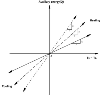
The rate of supply of heat produced by the proportional controller is modelled as proportional to the difference be- tween the set-point temperature and the room air temperature as:

Q〓G (T

－T

) (12)

Thus, if the room air temperature is very low, the heating source will work hard to overcome the temperature differ- ence (i.e. T

－T

). However, as the actual room air temper- ature (T

) approaches the set-point temperature (T

), the

output of the energy source decreases, there by preventing overshoot (Winn, 1982).

Fig. 3 represents the logic of this controller. As shown in the Figure, the slope of the line, G, is referred to as the con- troller gain. The disadvantage of the proportional controller, as illustrated, is that it would cause the energy source to op- erate continuously. At low energy rates, this results in inef- ficiency of the heating plant. The heating region or the cooling region in the Figure is determined depending upon the positive or the negative sign of (T

－T

). There is no dead band in the proportional controller in this study.

In many problems, the number of dimensional variables and parameters is large. Non-dimensionalization can be used to arrange these quantities into a smaller number of parame- ters. The physically significant parameters appear either in the differential equation or in boundary or initial conditions through a non-dimensionalization.

the solution can be represented in non-dimensional para- meterized form as follows:

T 〓T (x′ , t′ , Fo, Bi

, Bi

, âLS*/(kDT), DT

/DT,) QL

/(C

aDT), inital conditions) (13) where the two Biot numbers are:

Bi

〓h

L/k (14)

Fig. 2. On-off controller system. Fig. 3. Proportional controller system.

Bi

〓h

L/k (15)

Laplace transform solution

The Laplace transform approach was adopted, and proved to be successful although the inversion from the Laplace do- main to the real time domain was extremely complicated due to higher order poles. The Laplace transform method lends itself particularly well to the solution of linear, time-depen- dent problems. A transformation of the time variable essen- tially removes time from the transformed problem, rendering it easier to solve than the original equation. The formulation of the no auxiliary energy case can be easily obtained by set- ting Q in equation (5) to zero. This yields the“free re- sponse ”of the building.

Many excellent references exist on the Laplace transform technique. The reader is referred to Carslaw and Jaeger (1959) for its application to thermal problems. As the tech- nique is well known, only an outline of the solution proce- dure will be given here. The development of the solution begins via transformation of equation (1) to the Laplace do- main, s, as follows:

d

T (x, s)/dx

－sT (x, s)/a + ( ∑

n〓0

a

/x

)/a〓0 (16) Boundary conditions, equations (2) and (3), transformed to the s-domain as follows:

dT (x, s)/dx (x 〓0)〓－âS* (s)/k－h

(T

(s) －T

(s))/k (17) dT (x, s)/dx (x 〓L)〓h

(T

(s) －T

(s))/k (18) As the right-hand side of equation (1) is first order in time, the initial condition is incorporated in equation (16) in the process of transformation. Equation (5) for the air tempera- ture is transformed to:

(s + b) T

(s) －T

〓MT

(s) + I ′ T

(s) + Q/(C

s) (19) where:

M〓h

A/C

(20)

b〓M + I ′ (21)

The weather data, equations (10) and (11), are transformed

to:

S* (s) 〓b

/s +

∑

i－1

[(b

(s cosF

－w

sinF

)

+ c

(s sinF

+ w

cosF

))/s

+ w

] (22) T

(s) 〓d

/s +

∑

i－1

[(d

(s cosF

－w

sinF

)

+ e

(s sinF

+ w

cosF

))/s

+ w

] (23) Equations (16) through (23) require solution simultane- ously to obtain expressions for the wall temperature profile and the room air temperature in the Laplace domain. The so- lution in the transformed domain for the wall temperature profile is:

T (x, s)〓A (s) cosh (px) + B (s) sinh (px) + k

(s) + K

(s) x + K

(s) x

+ K

(s) x

+ K

(s) x

(24) T

(s) 〓[T

+ MT

(s) + I ′ T

(s) + Q/(C

s)]/(s +b) (25) The inversion can be obtained using a Bromwich contour theory based on Carslaw and Jaeger (1959). The form of the wall temperature as a function of time is:

T (x, t) 〓 ∑

m〓1

[(A

/C

) EXP ( －ah

t) cos (h

x) + (B

/C

) EXP ( －ah

t) sin (h

x))

+

11

i〓1

∑ [x

(x) cos (w

t) + x

(x) sin (w

t)] + f (x,t) (26) The form of the room air temperature as a function of time is:

T

(t)〓 ∑

m〓1

[(A

/D

) Mcos (h

L) EXP (－ah

t) + (B

/D

) Msin (h

L) EXP (－ah

t) +

11

i〓1

∑ [k

cos (w

t) + k

sin (w

t)] + f

(x) + K

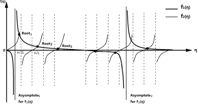
(27) where h

is the m

root of the characteristic equation, and Fig. 4 are showing these roots.

tan (Lh

) 〓[－h

K

]/K

(28)

The only the difference between the proportional con- troller and the on-off controller is in the form of Q, In this instance equation (5) becomes:

C

dT

/dt 〓－h

A (T

－T

) －C

′I (T

－T

) + G (T

－T

)

(29)

The governing equation, boundary conditions, and condi- tion are the same as for the on-off controller. Although only the auxiliary energy term is replaced, the solution for this case differs from the solution for the on-off controller.

Results and discussion

The solution procedure is selected to yield a daily simula- tion which is independent of the (arbitrarily selected) initial condition. This is done by simulating over a sufficient num- ber of identical days until the net daily internal energy stored in the wall is less than 0.25%. Generally, 7 or 8 iterations (days of simulation) are required to converge, depending on the house and the weather data. Energy loads are calculated and listed in Table 3 and Table 4, and there is not much dif- ference in energy consumption load for these two cases.

Our results are calculated under the assumption that each of the days used in this study is an average day, i.e. that the days preceding and following a given day are identical to the given day. We now turn our attention to a thought experi- ment for an alternate situation, that of several consecutive low solar radiation days followed by several consecutive high solar radiation days. The heavyweight structure will be able to store and release significant energy from one day to

the next. The fact that the simulations took eight (or so) days to converge lend credence to this. In such cases, the model would have to be exercised for the full period our approxi- mate model is not valid in these cases.

In order to study interactions between the house compo-

Table 3. Energy consumption loads (on-off controller)

Table 4. Energy consumption loads (proportional controller, G〓

250 W/°C)

City, month, house # Energy consumption load (MJ/day) Busan, Aug., #1

Busan, Aug., #2 Busan, Jan., #1 Busan, Jan., #2 Seoul, Aug., #1 Seoul, Aug., #2 Seoul, Jan., #1 Seoul, Jan., #2

2.23 1.19 4.35 4.13 3.80 2.75 8.43 7.21

City, month, house # Energy consumption load (MJ/day) Busan, Aug., #1

Busan, Aug., #2 Busan, Jan., #1 Busan, Jan., #2 Seoul, Aug., #1 Seoul, Aug., #2 Seoul, Jan., #1 Seoul, Jan., #2

2.30 1.04 4.72 4.15 4.00 2.95 9.25 7.90

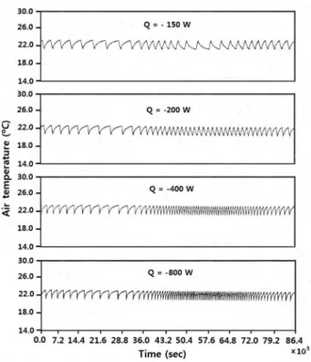
nents and the control, the room air temperature variations for four different Q’ s are plotted for different houses, cities, and months.

As shown in Fig. 5 and Fig. 6, the total number of cycles decreases as the absolute value of Q decreases. The result in- dicates that there is not much difference in energy load for each case even though Q changes drastically. This is because energy inefficiencies due to cycling are not considered in this study. Choosing an optimum Q will be an important matter in practice as we seek a balance between comfort and energy usage.

As explained before, the output of the auxiliary energy source in this case is proportional to the difference between

#1, Busan, Aug.)

Fig. 6. Room air temperature variation for four different Q’s (house

#1, Seoul, Jan.)

Fig. 7. Room air temperature variation for five different G ′s (pro- portional controller, house #1, Busan, Aug.)

Fig. 8. Room air temperature variation for five different G ′s (pro- portional controller, house #1, Seoul, Jan.)

the actual room air temperature and the set-point tempera- ture. G is referred to as the controller gain. Several values of G are tested to obtain room air temperature trajectories, When too small a value of G is used, the room air temperature lies between the comfort range and the sol-air temperature. This occurs because Q is not large enough to heat (or cool) the room air to approach T

. Appropriate values of G are deter- mined after several trials for two houses.

Fig. 7 and Fig. 8 show the room air temperature variation for five different G ′s. House #1 is chosen for application.

Busan in August and Seoul in January are used for weather conditions. A small G, such as 50 W/。 C, results in tempera- tures far removed from the set-point temperature, while using a large G makes the room air temperature very close to T

.

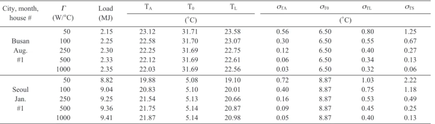
A high temperature swing is observed in house #1. This swing increases as G decreases. Table 5 shows all these com- parisons. The comfort level increases as G increases, but this results in greater energy input. s in the Table is standard de- viation.

Average values for T

, T

, and T

for proportional control such as 250 W/ 。C of G are also presented in Table 6. Again,

a wall mass effect on the thermal behavior of a house exists in mild weather such as Busan but not so in extreme weather such as Seoul, which is the same conclusion reached in the case of on-off control.

Conclusions

An analytical solution based on a rigorous mathematical model has proved effective in comparing the energy con- sumption in two different types of houses and weather con- ditions. Useful information has been obtained in the categories of energy usage, comfort, and auxiliary system cycling rate.

There is a significant wall mass effect on the thermal per- formance of a building in mild weather conditions such as Busan. This effect is due to the thermal wave (due to ambient variability) penetrating the structure, and interacting in a non- linear fashion with the auxiliary energy system controller.

Buildings of heavyweight construction with insulation (house #2) show the highest contort level in Busan. This is true both in terms of room air temperature, and mean radiant temperature as both fluctuate very little.

There is not much difference in energy load for each case even though Q changes drastically. This is because energy inefficiencies due to cycling are not considered in this study.

A proportional controller provides the highest comfort levels in comparison with buildings using a on-off controller. Com- fort can be increased by using a smaller dead band in the on- off controller. As far as energy consumption loads are concerned, there is no big difference between the propor- tional controller and the on-off controller.

Table 5. Comparison when different G ′s are used for proportional control

Table 6. Average temperatures (proportional controller) City, month,

house #

G (W/°C)

Load (MJ)

__TA

__T0

__TL sTA sT0 sTL sTS

(。C) (。C)

Busan Aug.

#1

50 100 250 500 1000

2.15 2.25 2.30 2.33 2.35

23.12 22.58 22.25 22.12 22.03

31.71 31.70 31.69 31.69 31.69

23.58 23.07 22.75 22.61 22.56

0.56 0.30 0.12 0.06 0.03

6.50 6.50 6.50 6.50 6.50

0.80 0.55 0.40 0.34 0.32

1.25 0.67 0.27 0.13 0.06

Seoul Jan.

#1

50 100 250 500 1000

8.82 9.04 9.25 9.36 9.41

19.88 20.83 21.54 21.75 21.87

5.08 5.10 5.13 5.14 5.14

19.10 20.01 20.66 20.87 20.98

0.72 0.40 0.16 0.09 0.05

8.87 8.87 8.87 8.87 8.87

1.03 0.75 0.53 0.45 0.40

2.22 1.18 0.49 0.25 0.13

City, month, house # ^__TA

__T0

__TL

Busan, Aug., #1 Busan, Aug., #2 Busan, Jan., #1 Busan, Jan., #2 Seoul, Aug., #1 Seoul, Aug., #2 Seoul, Jan., #1 Seoul, Jan., #2

21.97 21.96 21.82 21.82 22.15 22.13 21.42 21.44

21.70 21.42 10.20 9.77 28.50 28.19 5.15 4.76

21.95 21.93 21.54 21.56 22.45 22.41 20.56 20.68

Finally, it appears that both mass and wall insulation are important factors in the thermal performance of houses in general, but their relative merits should be decided in each building by a strict analysis of the building layout, weather conditions, site location.

Acknowledgment

This work was supported by a Research Grant of Pukyong National University (C-D-2013-0428)

References

Brigham EO. 1974. The fast Fourier transform. Prentice Hall, Inc., New Jersey, USA, 25－150.

Buffington DE. 1975. Heat gain by conduction through exterior walls and roofs-transmission matrix method. ASHRAE Trans- actions 81, Part 2, 89－101.

Carslaw HS and Jaeger JC, 1959. Conduction of heat in solids. Ox- ford Press, Great Britain, 92－326.

Christensen C and Perkins P. 1981. Effect of internal gain assump- tions in building energy calculations. Solar Engineering, 408－ 414.

Gadgil A, Bauman F and Kammerud, R. 1982. Natural convection in passive solar buildings: experiments, analysis and results.

Passive Solar J 1 (1). 28－40.

Incropera PI, Dewitt DP, Bergman TL and Lavine AS. 2013. Foun- dations of heat transfer. John Wiley & Sons, Inc., New York, USA, 111－194.

Kreyszig E. 2011. Advanced engineering mathematics. John Wiley & Sons, Inc., New York, USA, 540－600.

Kusuda T. 1976. Procedure employed by the ASHRAE task group for the determination of heating and cooling loads for building energy analysis. ASHRAE Transactions 82 (1), 305－314.

Marks’ standard handbook for mechanical engineers. 1978. Mc- Graw-Hill, Inc. New York, USA, 4－1〜4－82.

Mitalas GP and Stephenson DG. 1967. Room thermal response fac- tors. ASHRAE Transactions 73 (1), III.2.1－III.2.10.

Modest MF. 1993. Radition heat transfer. McGraw-Hill, Inc. New York, USA, 483－500.

Oosthuizen PH and Naylor D. 1999. Introduction to convective heat transfer analysis. McGraw-Hill, Inc. New York, USA, 426－ 477.

Peavy BA, Powell FJ and Burch, DM. 1973. Dynamic thermal per- formance of an experimental masonry building. U.S. National Bureau of Standards, Build Sci 45, 112－136.

Sodha MS, Kaur B, Kumar A and BansaL, NK. 1986. A Compari- son of the admittance and Fourier methods for predicting heat- ing/cooling loads. Solar Energy 36 (2), 125－127.

Stephenson DG and Mitalas GP, 1967. Cooling load calculations by thermal response factor method. ASHRAE Transactions 73 (1), III.1.1－III.1.7.

Winn CB. 1982. Controls in solar energy systems,”Advances in Solar Energy, American Solar Energy Soc, Inc., 209－240.

2014. 7. 11 Received

2014. 8. 12 Revised

2014. 8. 26 Accepted