OrdinalEncoder based DNN for Natural Gas Leak Prediction
Dashdondov Khongorzul1, Sang-Mu Lee2, Mi-Hye Kim3*
1Researcher, Dept Computer Engineering, Chungbuk National University
2Ph.D. Course, Dept. Computer Engineering, Chungbuk National University
3Professor, Dept. Computer Engineering, Chungbuk National University
천연가스 누출 예측을 위한 OrdinalEncoder 기반 DNN
홍고르출1, 이상무2, 김미혜3*
1충북대학교 컴퓨터공학과 연구원, 2충북대학교 컴퓨터공학과 박사과정, 3충북대학교 컴퓨터공학과 교수
Abstract The natural gas (NG), mostly methane leaks into the air, it is a big problem for the climate.
detected NG leaks under U.S. city streets and collected data. In this paper, we introduced a Deep Neural Network (DNN) classification of prediction for a level of NS leak. The proposed method is OrdinalEncoder(OE) based K-means clustering and Multilayer Perceptron(MLP) for predicting NG leak.
The 15 features are the input neurons and the using backpropagation. In this paper, we propose the OE method for labeling target data using k-means clustering and compared normalization methods performance for NG leak prediction. There five normalization methods used. We have shown that our proposed OE based MLP method is accuracy 97.7%, F1-score 96.4%, which is relatively higher than the other methods. The system has implemented SPSS and Python, including its performance, is tested on real open data.
Key Words : Natural Gas, OrdinalEncoder, MLP, K-means, F1-score
요 약 대부분의 천연가스(NG)는 공기 중으로 누출 되며 그중에서도 메탄가스의 누출은 기후에 많은 영향을 준다.
미국 도시의 거리에서 메탄가스 누출 데이터를 수집하였다. 본 논문은 메탄가스누출 정도를 예측하는 딥러닝(Deep Neural Network)방법을 제안하였으며 제안된 방법은 OrdinalEncoder(OE) 기반 K-means clustering과 Multilayer Perceptron(MLP)을 활용하였다. 15개의 특징을 입력뉴런과 오류역전파 알고리즘을 적용하였다. 데이터 는 실제 미국의 거리에서 누출되는 메탄가스농도 오픈데이터를 활용하여 진행하였다. 우리는 OE 기반 K-means알고 리즘을 적용하여 데이터를 레이블링 하였고 NG누출 예측을 위한 정규화 방법 OE, MinMax, Standard, MaxAbs.
Quantile 5가지 방법을 실험하였다. 그 결과 OE 기반 MLP의 인식률이 97.7%, F1-score 96.4%이며 다른 방법보다 상대적으로 높은 인식률을 보였다. 실험은 SPSS 및 Python으로 구현하였으며 실제오픈 데이터를 활용하여 실험하였 다.
주제어 : Natural Gas, OrdinalEncoder, MLP, K-means, F1-score
*This research was financially supported by the Ministry of Trade, Industry, and Energy (MOTIE), Korea, under the “Regional Specialized Industry Development Program (R&D, P0002072)” supervised by the Korea Institute for Advancement of Technology (KIAT).
*Corresponding Author : Mi-Hye Kim([email protected]) Received August 19, 2019
Accepted October 20, 2019
Revised October 2, 2019 Published October 28, 2019
1. Introduction
The Natural gas mostly methane a powerful greenhouse gas is wasting a source of energy. It is a significant contributor to climate change.
The major health concern about outdoor methane leaks is that they contribute to smog, which aggravates asthma and other respiratory conditions.
The researchers studied a better awareness of the impact of methane leaks is the first step, and this mapped pilot project is started[1-3]. We use open-source data on this study of Weller[1].
When natural gas leaks into the air, it's a big problem for the climate. So EDF and Google Earth Outreach teamed up to build a faster, cheaper way to find and assess leaks under our streets and sidewalks. They used Google Street View cars and methane sensors to detect leaks under city streets and collected data tested this new approach as part of a pilot program in a dozen cities across the U.S and in collaborations with PSE&G and Consolidated Edison[1-3].
Methane level (ppb)[4]
Detection measurement range of CH4 (ppm)[5]
Estimated leak flow rate(g min)[6]
Low (<1800ppb)
Low (<4.5ppm)
Low (<1.6 g min^-1) Medium
(1800~2600ppb)
Medium (4.5ppm~9x10⁴ppm)
Medium (1.6~26 g min^-1) High
(>2600ppb)
High (> 9x10⁴ppm)
High (>26 g min-1) Table 1. CH4 leak detection measurement and
estimated rate range.
There are few related works, which have been done to defined natural gas leak emission level.
Methane levels ranged between about 1800 and 2600 parts-per-billion(ppb) throughout, were consistent with the wind direction in Mcmanus[4]. This is consistent with the wind direction. Also[7-10] identified the primary as discriminated small leaks <6Lmin−1 from medium leaks (6−40Lmin−1) and a high bin (>40Lmin−1) for leaks estimated level.
We used a data survey from the Los Gatos Research CH4 analyzer's high-sensitivity mobile and portable survey[6]. There was more than a sequence of amount difference in the sensitivity of a device used to measure CH4 levels.
Therefore, this CH4 analyzer was susceptible to just a rare parts-per-billion(ppb) withdrawal from the background, LDCs frequently use hand-held sensors with parts-per-million(ppm) level sensitivities. In this study CH4(ppm) is the target feature, used OE methods for the real number to labeling feature for the data pre-processing part. The measurement and estimated leak flow rate levels of CH4 referred to as Table 1.
2. System overview
2.1 Architecture
In this paper, we study neural network architectures that are OE normalization and k-means cluster algorithm used in the data labeling prediction by low, medium and high.
The feedforward MLP network is used frequently in classification prediction[11]. We modeled architecture as follows, their indicator device speed and wind speed data give into input layers.
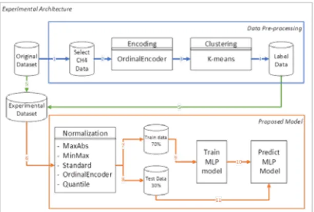
methane leaked label data predicted in the output layer. Proposed experimental architecture is presented in Fig. 1 This experiment is divided into 2 part. First part is the data pre-processing illustrated by blue line another one is proposed predicted model illustrated by the orange color line. Step 1 is we extracted (selected) CH4 data from the original dataset, step 2 is the encoding OE on the CH4, step 3 is the k-means clustering for the CH4 using SPSS IBM24 program and labeling by low, medium and high in the data pre-processing part. Next, step 5 is the develop experimental dataset which combined original dataset excluded CH4 and labeled data. Step 6 is the implemented normalizing five methods as
OE, MinMax, Standard, MaxAbs, and Quantile.
Step 7 and 8 are divided train and test part of data sets. Step 9 trains data will implement in train MLP model and prediction is shown in step 10. Finally step 11 is test data will predict the MLP model. We proposed to make a label for CH4 (ppm) value on the data preprocessing. In this case, we suggested OE methods before clustering data on our dataset.
Fig. 1. Experimental Architecture of Proposed model
2.2 Datasets
Methane concentration was measured by the Picarro CH4 sensor and the Google Street View Car. Below is the list of fields from the raw data the methane leaks data detected from the mobile device-based methane survey data in Weller[1], Zachary[6]. We have 3 kinds of datasets. Firstly, original dataset has 15 features including
“CavityPressure”, “CavityTemp”, “DasTemp”,
“EtalonTemp”, “WarmBoxTemp”, “CH4”,
“GPS_ABS_LAT”, “GPS_ABS_LONG”, “WS_WIND_LON”,
“WS_WIND_LAT”, “WIND_N”, “WIND_E”,
“WIND_DIR_SDEV”, “CAR_SPEED”. Secondly, we selected target feature of methane(CH4) from the original dataset. Thirdly, the experimental dataset has 15 features including “label” feature on the original dataset deposed CH4. Fig. 2 shows a comparison between original, OE and other normalization of CH4.
Fig. 2. Plot of OE and other normalization of CH4
2.3 Proposed methods
The generalization of deep neural network architecture can be evaluated by modifying the number of adaptive parameters(weights and biases) in the network. In our previous work compared architectures[12]. Therefore, in this paper we selected DNN architecture as Hidden Layer (HL) = 20 and node = 20, solver given by
“adam”, activation has ‘relu’.
Fig. 3. The proposed DNN architecture
MLPs are supervised models, meaning that for the network to predict the correct output values, it must be allowed to learn on a training dataset for which the correct outputs are already
known[13-14]. The goal of this learning is for the network’s predictions to be as close to the true outputs as possible. [15-16] has compared the accuracy of a deviation-based classification, Bayesian and SVM classification algorithms.
Proposed prediction network architecture is presented in Fig. 3.
In this paper, we compared some normalization methods performance for the data pre-processing on the DNN prediction.
a. OrdinalEncoder : Encode the categorical features as an integer array. The input should be integers or strings array, expressing the values taken on by discrete categorical features. The features are changed to ordinal integers as a single column of integers (0 to n-1) per feature.
Where n is the number of categories. We implemented the OE to a set of attributes and issued the setting between numerical values and categories ‘low', 'medium' and 'high'.
b. MinMax : Min-max normalization is commonly known as feature scaling where the values of a data feature's numeric range, an attribute, are reduced to a scale between 0 and 1. Therefore, in order to calculate z, the normalized value of a member of the set of observed values of X as follows:
max min
min
(1) where, min and max are the minimum and maximum values in X given its range.
c. MaxAbs : This estimator scales and translates each feature separately such that the maximal absolute value of each feature in the training set will be 1. Only on positive data, this scaler behaves similarly to MinMaxScaler and therefore also be upset from the presence of large outliers. The maximum absolute value is scaled by each feature.
d. Standard : Standardization is the process of transforming a variable to one with a mean of 0 and a standard deviation of 1.
(2) where, μ is the mean, is the standard deviation.
e. Quantile : QuantileTransformer (QT) uses a non-linear transformation, that every feature's probability density function (pdf) will be displayed to a uniform distribution. In this case, all data will be plotted in the range[0, 1], therefore, the outliers which cannot be differentiated anymore from the inliers. QT is strong to outliers in the sense that adding or removing outliers in the training set will allow nearly the same transformation on extending data. But contrary to QT will automatically reduce all outliers by setting them to the previously defined range boundaries (0 and 1).
3. Evaluation metrics
The data evaluation of this paper was performed using F1-score, accuracy and mean squared error (MSE). In Fig. 4 shows the model of confusion matrix. From Fig. 4 we can find precisions and recall as follows:
Pr
and
(3) We have studied on the multi-label case, there the average of the F1-score of each label with weighting depending on the average parameter as Eq. (5). The harmonic mean of precision and recall for F1-score is the follows:
Fig. 4. Model of confusing matrix
Pr
·Pr· (4)
· (5) where W – weight of support.The accuracy is an evaluation measure of the amount of closeness of calculated value to its actual value. Accuracy equals to the sum of true positive fraction and true negative fraction among all the test data.
(6)
Additionally, mean squared error (MSE) for the predicted leaks to relative to actual values was used:
(7) With X and Y being the actual and predicted values for the i, j - th data point, respectively, and m and n are the number of observations. In our case, m is a number of data and n is predicting methane.4. Experimental Results
The dataset is selected on 20170314, between 12:33:59AM to 12:34:02AM hours has “TR0314-1”, 8:34:03PM to 9:34:07PM hours has “TR0314-2”, 9:34:07PM to 9.48:41PM hours has “TR0314-3”
and 9:57:00PM to 10:07:53PM hours has
“TR0314-4” for Sample_Raw open data. In the experiment, we set λ = 0.001. Architecture solver given by “adam”, activation has ‘relu’. In the default setting of training and testing set (training set has 70%, the testing set has 30%).
The training set has divided 80% by training, 20%
by validation sets.
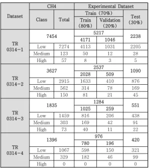
The descriptive analysis has described in Table 2. Recall, the class has labeled by OE based k-means clustering method by low, medium and high implemented in the SPSS IBM24. The comparison results of the normalization performance are
shown in Table 3, in which a classification accuracy, F1-score and MSE for the testing data, respectively. There can help us know how the models perform when the normalized threshold is not selected properly. This analysis does not include feature selection. The learning rate is set to η = 0.001. MLP predicts leakage on proposed architecture with accuracy 97.6%, F1-score 96.39% and MSE 0.047 on the OE; accuracy 93.83%
and F1-score 95.5% and MSE 0.06 on the MaxAbs, better than other normalization methods for TR0314-1. The F1-score can be performed as a
Dataset
CH4 Experimental Dataset
Class Total
Train (70%)
Test (30%) Train
(80%)
Validation (20%)
TR 0314-1
7454 5217
4171 1046 2238
Low 7274 4113 1031 2205
Medium 123 50 12 28
High 57 8 3 5
TR 0314-2
3627 2537
2028 509 1090
Low 2915 1633 410 876
Medium 562 314 78 169
High 150 81 21 45
TR 0314-3
1835 1284
1025 259 551
Low 1459 816 206 438
Medium 303 169 42 91
High 73 40 11 22
TR 0314-4
1396 976
780 196 420
Low 1067 598 150 321
Medium 329 182 46 99
High 0 0 0 0
Table 2. Descriptive statistics for CH4 and Experimental Dataset
Ordinal
Encoder MinMax Standard MaxAbs Quantile
TR 0314-1
F1 0.9639 0.3709 0.36831 0.9550 0.1735 ACC 0.9767 0.2390 0.2368 0.9383 0.1054 MSE 0.047 0.76 0.7631 0.061 0.9
TR 0314-2
F1 0.7240 0.7213 0.7235 0.7235 0.7235 ACC 0.7568 0.8036 0.8045 0.8045 0.8045 MSE 0.3532 0.3201 0.3192 0.3192 0.3192
TR 0314-3
F1 0.5893 0.6876 0.6930 0.3808 0.7365 ACC 0.5716 0.7622 0.7658 0.3157 0.8094 MSE 0.6188 0.3956 0.3539 0.809 0.3103
TR 0314-4
F1 0.6418 0.6621 0.6621 0.6874 0.6562 ACC 0.7238 0.7642 0.7642 0.7380 0.7523 MSE 0.2761 0.2357 0.2357 0.2619 0.2476 Table 3. Comparison of normalizations for the prediction
evaluation
weighted harmonic mean of the precision and where an F1-score gets its best value at 1 and the worst score at 0.
5. Conclusion
In this paper, we introduced the classification method of a prediction based MLP. The methane leaked class labeled by k-means algorithms.
The proposed method is OE based K-means clustering and MLP for predicting methane leak.
The 15 features are the input neurons and the backpropagated errors associated with the hidden neurons. Extensive computer simulations used real open data case of USA street for methane leak that the proposed method presents better or equivalent results than estimation rate of the leak. In this paper, we propose the OE method for labeling target data using k-means clustering and compared normalization methods performance for methane leak prediction. There five normalization methods used as OE, MinMax, Standard, MaxAbs, and Quantile. We have shown that our proposed OE based MLP method is accuracy 97.7%, F1-score 96.4% and MaxAbs accuracy 93.8% and F1-score 95.5% which is relatively higher than the other methods. The system has implemented SPSS IBM24 and Python, including its performance, is tested on real open data. In future work, we will predict based on the dimensionality reduction methods use the Korean NG data.
REFERENCES
[1] Z. D. Weller, D. K. Yang & J. C. von Fischer. (2019).
An open source algorithm to detect natural gas leaks from mobile methane survey data. PLOS ONE, 14(2), e0212287.
DOI:10.1371/journal.pone.0212287
[2] J. Wanga et al. (2019). Machine Vision for Natural Gas Methane Emissions Detection Using an Infrared Camera. arXiv preprint, arXiv:1904.08500v1
[3] L. Salhi et al. (2019). Early Detection System for Gas Leakage and Fire in Smart Home Using Machine Learning. 2019 IEEE International Conference on Consumer Electronics (ICCE). (pp. 1-6). Las Vegas : IEEE.
DOI: 10.1109/ICCE.2019.8661990
[4] J. H. Mcmanus et al. (1996). Methane emission measurements in urban areas in Eastern Germany, Journal of Atmos Chem, 24, pp. 121-140.
DOI: 10.1007/BF00162407
[5] J. Wilkinson et al. (2018). Measuring CO2 and CH4 with a portable gas analyzer: Closed-loop operation, optimization and assessment, PLOS ONE, 13(4), e0193973.
DOI: 10.1371/journal.pone.0193973.
[6] D. W. Zachary et al. (2018). Vehicle-Based Methane Surveys for Finding Natural Gas Leaks and Estimating Their Size: Validation and Uncertainty, Environmental Science & Technology, 52(20), pp. 11922-11930.
DOI: 10.1021/acs.est.8b03135
[7] F. H. Margaret et al. (2016). Fugitive methane emissions from leak-prone natural gas distribution infrastructure in urban environments, Environmental Pollution, 213, 710-716.
[8] Joseph C et al. (2017). Rapid, Vehicle-Based Identification of Location and Magnitude of Urban Natural Gas Pipeline Leaks, Environmental Science &
Technology, 51(7), 4091-4099 DOI: 10.1021/acs.est.6b06095
[9] E. K. Chandler, P. R. Arvind & R. B. Adam. (2016).
Comparing Natural Gas Leakage Detection Technologies Using an Open-Source “Virtual Gas Field” Simulator.
Environ. Sci. Technol. 50(8), 4546-4553.
DOI: 10.1021/acs.est.5b06068
[10] Brian K. Lamb et al. (2015). Direct Measurements Show Decreasing Methane Emissions from Natural Gas Local Distribution Systems in the United States, Environ. Sci. Technol. 49(8), 5161-5169.
DOI: 10.1021/es505116p
[11] P. Kaur & T. Choudhury. (2016). Early detection of SF6 gas in gas insulated switchgear, 7th India Int.
Conf. on Power Electronics (IICPE). (pp. 1-6). Patiala : IICPE.
[12] D. Khongorzul, M. H. Kim & S. M. Lee, (2019m July).
Classification using the Multilayer Perceptron prediction for Natural Gas leak. The 9th Int. Conf. on Conv. Techn.. (pp. 553-554). Jeju : ICCT.
[13] Matthew Barriault et al. (2018, May). Quantitative Natural Gas Discrimination For Pipeline Leak Detection Through Time-Series Analysis of an MOS Sensor Respons, Proc. of The Canadian Society for Mechanical Engineering Int. Congress, Toronto : CSME.
[14] Z. Xiaojun et al. (2016). MLP Neural Network Based Gas Classification System on Zynq SoC, IEEE Access, (4), 8138-8146.
DOI: 10.1109/ACCESS.2016.2619181
[15] Jin-Hee Ku. (2017). A Study on the Machine Learning
Model for Product Faulty Prediction in Internet of Things Environment. Journal of Convergence for Information Technology, 7(1), 55-60.
DOI: 10.22156/CS4SMB.2017.7.1.055
[16] Yong-Bae Lee. (2014). Classification Accuracy by Deviation-based Classification Method with the Number of Training Documents. Journal of Digital Convergence, 12(6), 323-332.
DOI: 10.14400/JDC.2014.12.6.325
홍 고 르 출(Khongorzul Dashdondov) [정회원]
․ 1998년 6월 : 몽골국립대학교 수학 과(이학사)
․ 2000년 12월 : 몽골국립대학교 수학 과(이학석사)
․ 2013년 8월 : 충북대학교 전파통신공 학과(공학박사)
․ 2017년 3월 ~ 현재 : 충북대학교 컴퓨 터공학과 연구원
․ 관심분야 : Probability and Statistics, Queueing theory, Image processing, Machine Learning
․ E-Mail : [email protected]
이 상 무(Sang Mu Lee) [정회원]
․ 2012년 2월 : 충북대학교 컴퓨터공 학과(공학사)
․ 2014년 2월 : 충북대학교 컴퓨터공학 과(공학석사)
․ 2014년 9월 ~ 현재 : 충북대학교 컴퓨 터공학과 박사 재학
․ 관심분야 : Machine Learning, Pattern Recognition, Gesture Recognition
․ E-Mail : [email protected]
김 미 혜(Mi-Hye Kim) [정회원]
․ 1992년 2월 : 충북대학교 수학과 (이학사)
․ 1994년 2월 : 충북대학교 수학과 (이 학석사)
․ 2001년 2월 : 충북대학교 수학과 (이 학박사)
․ 2004년 9월 ~ 현재 : 충북대학교 컴 퓨터공학과 교수
․ 관심분야 : 빅데이터, 기능성 게임, 유비쿼터스 게임, 플랫폼, 퍼지측도 및 퍼지적분, 제스츄어 인식
․ E-Mail : [email protected]