http://dx.doi.org/10.7840/kics.2014.39A.5.244
HMM기반 소음분석에 의한 엔진고장 진단기법
레 찬 수, 이 종 수°
Engine Fault Diagnosis Using Sound Source Analysis Based on Hidden Markov Model
Le Tran Su, Jong-Soo Lee° Abstract
The Most Serious Engine Faults Are Those That Occur Within The Engine. Traditional Engine Fault Diagnosis Is Highly Dependent On The Engineer'S Technical Skills And Has A High Failure Rate. Neural Networks And Support Vector Machine Were Proposed For Use In A Diagnosis Model. In This Paper, Noisy Sound From Faulty Engines Was Represented By The Mel Frequency Cepstrum Coefficients, Zero Crossing Rate, Mean Square And Fundamental Frequency Features, Are Used In The Hidden Markov Model For Diagnosis. Our Experimental Results Indicate That The Proposed Method Performs The Diagnosis With A High Accuracy Rate Of About 98% For All Eight Fault Types.
Key Words : Hmm, Engine Fault, Mfcc, Rms, Bayes
First Author : School of Electrical Engineering, University of Ulsan, 93 Daehak-ro, Nam-gu, Ulsan 680-749, Korea, 학생회원
° Corresponding Author : School of Electrical Engineering, University of Ulsan, 93 Daehak-ro, Nam-gu, Ulsan 680-749, Korea, 종신회원
논문번호:KICS2014-03-095, Received March 19, 2014; Revised May 8, 2014; Accepted May 8, 2014
Ⅰ. Introduction
Precise diagnose of engine faults has long been required for engine protection and safety, but current diagnosis techniques fledged to satisfy engine users have not produced satisfactory results. Engine products are advancing fast, but the diagnosis technique is not. Technicians have been relying on their experimental adroitness on diagnosing faults.
Diverse engine sounds from a variety of vehicle brands might mislead even an experienced technician in identifying faults. This kind of diagnose routine must be replaced with a new sophisticated technique keeping up with IT solution techniques. A remote diagnosis service should be possible at any time and any place.
Industrial systems with higher performance, safety
and reliability have increased the need for fault diagnosis with better precision. Precise fault diagnosis has also taken an important role in process monitoring systems. During the last two decades, various sensors have been developed and employed for fault diagnosis systems by monitoring displacement, vibration, dynamic force, acoustic emission, temperature, sound analysis, etc.
The sound signal analysis is widely used for condition monitoring and fault diagnostics because it is a non-contact diagnosis method with effective usability. With the fast technical development in the signal processing area, various schemes based on Neural network[1], Support Vector Machine[2] and fuzzy logic[3], are proposed to diagnosis engine faults. Unfortunately, these methods are not suitable for non-stationary sound signal analysis[4]. In
addition, they are not able to reveal the inherent information of non-stationary sound signals. These methods provide a limited performance when we use a small dataset of sound signals for the learning phase[1-3]. In order to solve these problems we propose to take the HMM for motor engine fault diagnosis. The method uses the HMM model to consider engine startup characteristics. Data representing the engine startup under the nominal conditions are used to train the HMMs and thus, determine the HMM parameters. This is analogous to system identification methods used to develop empirical models based on neural networks.
From each engine sound data bit the nominal HMM model produces log-likelihood values (posterior probabilities) which represent the closeness of the nominal engine represented by HMM to the engine data. In a similar way, HMM models representing the engine startup under various faulty situations can be developed; these are the so-called fault HMM models. We extracted, from sound source, the MFCC feature, the zero crossing rates, the mean square and the fundamental frequency which are then used to build HMM. In our experiment, a set of eight common types of engine faults is used to evaluate the proposed method. They are Eccentricity, angular misalignment, parallel misalignment; Bowed rotor;
broken Rotor bar; Faulty bearing; Rotor unbalance;
and Phase unbalance. The experimental result indicated that the proposed method shows the high recognition rate of about 98%.
The remainder of this paper is organized as follows. Section II presents the brief technical background about HMM and MFCC features.
Section III elaborates on the scheme we propose.
Section IV shows our experimental results. Section V proposes further study to incorporate with the IT infrastructure by smartphone applications.
Ⅱ. Back Ground
2.1 Hidden Markov Model
This section gives a short introduction to HMMs.
The reader is referred to Rabiner[5] for more details
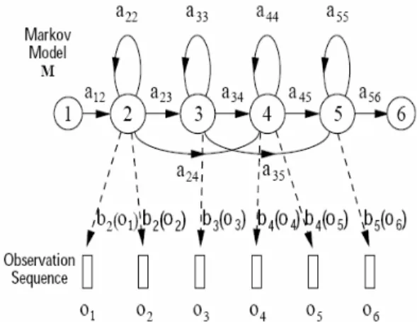
on HMMs. A hidden Markov model (HMM) is a statistical Markov model in which the system being modeled is assumed to be a Markov process with unobserved (hidden) states. A HMM can be considered the simplest dynamic Bayesian network.
In simpler Markov models (like a Markov chain), the state is directly visible to the observer, and therefore the state transition probabilities are the only parameters. In a hidden Markov model, the state is not directly visible, but output, dependent on the state, is visible. Each state has a probability distribution over the possible output tokens.
Therefore the sequence of tokens generated by an HMM gives some information about the sequence of states. Note that the adjective 'hidden' refers to the state sequence through which the model passes, not to the parameters of the model; even if the model parameters are known exactly, the model is still 'hidden'.
A hidden Markov model can be considered a generalization of a mixture model where the hidden variables (or latent variables), which control the mixture component to be selected for each observation, are related through a Markov process rather than independent of each other.
Each file from sound source is associated to each HMM model. It should then do some calculations of probability. Indeed, there is a series of observation O, the problem is to find the maximum value of P(M/O) (the probability of event model M generates the series of observations O).
Fig. 1. Hidden Markov Model
The Bayes formula
(1) In sound signal processing, the HMMs used are the left-right type. We advance always right (or one loops itself) and the model is a straight chain of states. The initial probabilities are fixed. We have a number of mathematical properties related to the facts that always makes a transition and that always gets a comment. It is, however, raises two crucial issues:
■ Recognition: Given a model and observations as to determine the optimal path according to a suitable criterion.
■ Learning: Given labeled examples, how to build HMM models and more specifically how to determine the initial probabilities of transition and observation. It is a first naive method to solve the probability of recognition.
Suppose we have models with N states and N observations, we can easily assess the likelihood of each model. If multiple paths are possible, we calculate a max on different paths for each model and between different models. For N states and T observations, it has complexity O (TNT).
To apply the hidden Markov model in the recognition of the sound source, we have to solve three problems:
■ First problem - Probability observation sequence:
We have an observation sequence and model is given. What is the probability for the controller characterized by the parameters P(O|λ)
■ Second problem - Recognition: There is sequence of observation sequence with a model is given.
What is the sequence of state the most probable that produced
■ Third problem – Learning: Given the observation sequence and a space of models found by varying the model parameters, what is the best model?
2.2 Mel-Frequency Cepstrum Coefficient Firstly, module signal processing performs the sound signal analysis on the short timeslots, of 10 to 30 ms. After this step, the signal is represented by acoustic parameter vectors that can discriminate
different sound sources, which reduces the amount of information and redundancy.
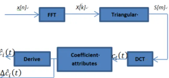
Actually, our ear is sensitive to frequencies of the sound signal and our hearing is linear with low frequencies (below 1000 Hz) and logarithmic with high frequencies (above 1000 Hz). So batteries triangular filters are varied linearly with low and high frequencies with logarithmic frequencies are used to set the tone. They help us to reduce the amount of information needed to analyze the sound signal. Fig. 2 presents scheme for calculating MFCC coefficients.
There are three main steps in MFCC process[6]:
► Take the Fourier transform (FFT) of (a windowed excerpt of) the input sound signal x[n] we obtain the spectrum of the sound signal X[k].
► Map the powers of the spectrum obtained above onto the mel scale, using triangular overlapping windows.
► Take the logs of the powers at each of the mel frequencies.
► Take the discrete cosine transform of the list of mel log powers, as if it were a signal.
► The MFCCs are the amplitudes of the resulting spectrum.
Fig. 2. Mel-Frequency Cepstrum Coefficient
Ⅲ. Proposed Method
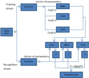
In this section, we propose a system model to detect the engine fault from sound source. The general model is shown in Fig. 3.
Structure of our proposed fault diagnosis system from sound source is shown in the following figure:
Signals of engine failures sound are recorded to files; the first stage is to extracting sound signals
Fig. 3. System structure recognition engine failures into features (parameters).
Feature extraction phase:
The sound signal is processed with a pre-emphasis filter then ignored the silence part. The filter function is
After that, the sound signal is divided into frames with length from 20 – 30ms. Each frame is multiplied with Hamming window to ensure the continuous of whole signal.
(2)
The output of this stage is a set of parameter vectors X = {X(k)} with X(k)= {x1,x2,..xN}. Each parameter vector has N dimensions. In this case, we have:
■ The number of coefficients is 13 MFCCs
■ The number of dynamic parameters (13 parameters derived first order, 13 parameters derived second order)
■ A coefficient of energy
■ RMS coefficient
■ A coefficient of zero crossing rate
■ A coefficient of variation of the fundamental frequency
The method to extract MFCCs parameters is described in the previous section.
The zero crossing rate is calculated as follow:
(3)
RMS·coefficient·RMS= (4)
Coefficient of variation of the fundamental frequency
(5)
In the diagram, we can find that the process of recognition of the sound source consists of two phases. This is the learning phase and the recognition phase:
Learning phase:
The set of parameters is used for building of HMMs. In recognition system engine failures using hidden Markov model, each engine failure is represented by an HMM, the parameters of this failure are used to train the corresponding HMM. In fact, the training process is the process of estimating the parameters to obtain the maximum probability P(O|λ). This process is performed repeatedly until the difference between two probability P(O|λ) has reached a threshold. The provided threshold is calculated based on the number of repetitions following a specified limit.
Recognition phase
The set of parameters is used as the input all HMM models and these models are trained in the previous learning phase. Using the second problem among three problems hidden Markov model, we can easily calculate the corresponding observation probabilities: P1...PK. selecting the probability which is the largest, for example, Pi, then the recognized fault is that the probability Pi represented.
Ⅳ. Experiment
In our experiments, we consider eight states of the activity of engine failure including:
■ amis – angular misalignment
Fig. 5. The signal states of the activity of motor
Fig. 4. Some pictures of engine failures
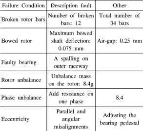
Failure Condition Description fault Other Broken rotor barsNumber of broken
bars: 12
Total number of 34 bars
Bowed rotor
Maximum bowed shaft deflection:
0.075 mm
Air-gap: 0.25 mm
Faulty bearing A spalling on outer raceway Rotor unbalance Unbalance mass
on the rotor: 8.4g Phase unbalance Add resistance on
one phase 8.4
Eccentricity
Parallel and angular misalignments
Adjusting the bearing pedestal Table 1. Failure description
Fig. 6. Experiment setup.
■ br – bowed rotor shaft
■ brb – broken rotor bar
■ fbo—faulty bearing (out race)
■ mun – rotor unbalance
■ nor – normal motor
■ pmis – parallel misalignment
■ pun – phase unbalance
In figure 3, we show some pictures of engine failure cases.
Detail description of faulty induction motors is defined in table 1.
In figure 4, we represent the wave form of sound signal from each state of engine failure.
Experiment setup
We setup the system to implement the experiment as figure 5. Each experiment is measured twenty times under full-load condition.
The parameters of system are configured as follow:
a1~a3 vibration signal (acceleration) maximum frequency : 8000kHz sample number : 16384uh time: 2.1333 s
The recognition system failures motor is installed well with relative accuracy. This justified the correction of the theory and the effectiveness of hidden Markov model in recognition of the sound source.
The detail of obtained recognition rate is presented in table 2. The preliminary results shown that, exception the unbalance status (phase and rotor) had a lower accuracy rate (≈ 92 – 93%), all other got a very high recognition rate (100%).
We also implemented the fault diagnosis process with neural network[1], SVM[2] for comparison. The result is shown in table 3. The comparison result indicated that our method provides a better result than the NN and SVM method (considering in case of number of files for learning phase is small). In
Failure type
Number of files for learning phase
Number of files for recognition
phase
Accuracy
Amis 6 13 100%
Br 6 13 100%
Brb 6 14 100%
Fbo 6 13 100%
Mun 6 13 92%
Nor 6 13 100%
Pmis 6 13 100%
Pun 6 30 93%
Table 2. Recognition result
Failure
type NN SVM HMM
Amis 96 98 100%
Br 95 98 100%
Brb 97 97 100%
Fbo 94 96 100%
Mun 90 91 92%
Nor 96 97 100%
Pmis 95 95 100%
Pun 90 91 93%
Table 3. Comparison result
this experiment, we kept all number of files in the learning and recognition phase the same as in the previous experiment.
Ⅴ. Conclusion
In this paper, we elaborate our method which diagnoses engine failure from sound source. We set up the test environment and implemented the algorithm with S/W. Our experimental results indicated that our method outperformed other methods such as NN and SVM in the recognition rate. The proposed system can recognize 8 different engine failures. The Hidden Markov model has been proved to be efficient in fault recognition of the sound source. However, in further research, the engine fault diagnosis system from sound source needs more complex functions such as: Recognition of most of types of sound sources; Identify in real time, recognition within a noisy environment.
It is difficult to solve these problems above, because it relates to several areas. To deal with
these challenges, we can develop the system in some directions: Building module filtering noise and spurious signals; divide sound sources into segments that have similar characteristics then research the characteristics of these segments.
The quick growth of smartphone use in recent years is creating a demand for applications. Based on the obtained result, we propose future work to apply our implementation on the Android smartphone. A set of induction motors tested both normal and faulty, to analyze sound signals recorded with a smartphone. Then, recorded data is analyzed by our Android application to identify healthy and faulty emissions status.
References
[1] H. Kumar, T. A. R. Kumar, M. Amarnath, and V. Sugumaran, “Fault diagnosis of antifriction bearings through sound signals using support vector machine,” J.
vibroengineering, vol. 14, no. 4, Dec. 2012.
[2] M. Paul, F. Corresponding, and Birgit Köppen-Seliger, “Fuzzy logic and neural network applications to fault diagnosis,” Int. J.
approximate Reasoning, vol. 16, no. 1, pp.
67-88, Jan. 1997.
[3] D. Sauter, N. Mary, F. Sirou, and A.
Thieltgen, “Fault diagnosis in systems using fuzzy logic,” in IEEE Proc. Control Appl., vol. 2, pp. 883-888, Aug. 1994.
[4] H. Bendjama, S. Bouhouche, and M. S.
Boucherit, “Application of wavelet transform for fault diagnosis in rotating machinery”, in Int. J. Machine Learning and Comput., vol. 2, no. 1, Feb. 2012.
[5] L. Rabiner, “A tutorial on hidden markov models and selected applications in speech recognition,” in Proc. IEEE, vol. 77, no. 2, pp. 257-286, Feb. 1989.
[6] L. Muda, M. Begam, and I. Elamvazuthi,
“Voice recognition algorithms using mel frequency cepstral coefficient (MFCC) and dynamic time warping (DTW) techniques,” J.
Comput., vol. 2, no. 3, Mar. 2010.
Le Tran Su
He received his bachelor’s degree in information systems and communication in 2005 from Hanoi University of Technology, Vietnam. In 2009, he received his master’s degree from University of Ulsan, Korea. He is currently working as a Ph.D. candidate in the Multimedia Applications Laboratory at the University of Ulsan in Korea. His research interests include image processing, parallel computing, and speech recognition.
Jong-Soo Lee
He received his bachelor’s degree in electrical engineering in 1973 from Seoul National University and his M.Eng. in 1981. In 1985, he was awarded his Ph.D. from Virginia Polytechnic Institute and State University in the US. He is currently working in the area of multimedia applications at the University of Ulsan in Korea. His research interests include the development of personal English cultural experience programs using multimedia applications and usability interface techniques to facilitate the acquisition of English language skills by Koreans.
He is also working on multimedia-based online TOEIC and brain-gymnastics training.