Generation Schemes
Yoon, Chongyul† Park, Joon-Seok*
···
Abstract
The finite element method(FEM) is proven to be an effective approximate method of structural analysis if proper element types and meshes are chosen, and recently, the method is often applied to solve complex dynamic and nonlinear problems. A properly chosen element type and mesh yields reliable results for dynamic finite element structural analysis. However, dynamic behavior of a structure may include unpredictably large strains in some parts of the structure, and using the initial mesh throughout the duration of a dynamic analysis may include some elements to go through strains beyond the elements' reliable limits. Thus, the finite element mesh for a dynamic analysis must be dynamically adaptive, and considering the rapid process of analysis in real time, the dynamically adaptive finite element mesh generating schemes must be computationally efficient. In this paper, a computationally efficient dynamically adaptive finite element mesh generation scheme for dynamic analyses of structures is described. The concept of representative strain value is used for error estimates and the refinements of meshes use combinations of the h-method(node movement) and the r-method(element division). The shape coefficient for element mesh is used to correct overly distorted elements. The validity of the scheme is shown through a cantilever beam example under a concentrated load with varying values. The example shows reasonable accuracy and efficient computing time. Furthermore, the study shows the potential for the scheme's effective use in complex structural dynamic problems such as those under seismic or erratic wind loads.
Keywords : structural engineering, structural dynamics, dynamically adaptive finite element mesh, finite element method
···
†책임저자, 정회원․홍익대학교 건설도시공학부 교수 Tel: 02-320-1478 ; Fax: 02-322-1244 E-mail: [email protected]
* 홍익대학교 토목공학과 박사과정
∙이 논문에 대한 토론을 2011년 2월 28일까지 본 학회에 보내주시 면 2011년 4월호에 그 결과를 게재하겠습니다.
1. Introduction
The finite element method (FEM) is proven to be an effective approximate method of structural analysis (Bathe and Wilson, 1976; Belytschko et al., 1996;
Cook et al., 1989; Reddy, 1993; Zienkiewcz et al., 2005). When the method is applied to dynamics analyzed in the time domain, the meshes may need to be modified at each time step as the finite element results of an analysis largely depend on the mesh and the element types used (Heesom and Mahdjoubi, 2001). Dynamic behavior of a structure may include unpredictably large strains in some parts of the structure, and if the initial mesh is used throughout the duration of a dynamic analysis, some elements may go through strains beyond the elements' reliable
limits during the analysis. Thus, the finite element mesh for a dynamic analysis must be dynamically adaptive, and considering the rapid process of analysis in real time, the dynamically adaptive finite element mesh generating scheme must be computationally efficient.
In this paper, a dynamically adaptive finite element mesh generation scheme for dynamic analysis of structures is described. An adaptive mesh generation process involves estimation of error given a mesh and generation of a new improved mesh based on the error (Choi and Jung, 1998; Choi and Yu, 1998; de Las Casa, 1988; Zienkiewcz and Zhu, 1987). The dynamically adaptive scheme uses computationally simple error estimation based on representative strain.
The mesh generating scheme combines the r-method
(moving an existing node) and the h-method (dividing an element into smaller elements). The scheme includes a check for limiting distortion for each element using the concept of shape factor that is easily computed for each shape. The dynamic analysis considered is in time domain, based on direct integration. As an example, an undamped cantilever beam modeled with four node quadrilateral isoparametric elements for plane stress is considered. The results of the analyses of the example show that the proposed dynamically adaptive finite element mesh scheme using the error estimation based on the representative strain, the r-h method, and the shape factor is efficient compu- tationally and have reasonable confidence level for complex dynamic problems in structural analysis.
2. Adaptive mesh scheme for dynamic analysis
2.1 Error estimation with representative strains
The results of a finite element analysis largely depend of the type of element and the mesh used. An adaptive mesh generation scheme attempts to automate the mesh generation and in the scheme, accuracy of error estimation of a given mesh is essential (Hwang, 1988; Jeong et al., 2003; McFee and Giannacopoulos, 2001; Ohnimus et al., 2001; Stampgle et al., 2001;
Yoon, 2005; Zhu et al., 1991).In general engineering problems, accurate solutions are not known and thus accurate error estimation is inherently a difficult problem. In addition, error estimation for adaptive mesh needs to be computationally efficient, especially for dynamic problems, since there are extensive additional computations needed for many aspects of adaptive mesh generation and analyses that follow.
Norm of a matrix is generally used to represent error of a mesh where the matrix includes values of stress, strain and displacements. The error in the domain Ω may be represented as follows:
(1)Here , are the exact solutions for stress and strain and , are the finite element solutions. The error defined in Eqs. (2~5) are the representative strain of element based on the standard deviations of the strains at the Gauss points in the element computed during the previous finite element analysis (Jeong and Yoon, 2003; Yoon, 2009). The z axis is not considered in planar problems, and the representative strain values of element are represented by the following equations:
(2)
(3)
(4)
×
(5)
Here, is the x directional standard deviation of the strain, is the number of Gauss points in
direction, is the directional strain of Gauss point , and
is the directional strain; ,
, ,
are the similar directional values and
, , , are the similar shear strain values. In addition, is the element area and is the total area of the mesh.
2.2 Dynamic analysis
The direct numerical integration in the time domain is used for the dynamic analysis. Specifically, the Newmark- method, a reliable explicit method widely used in dynamic structural analysis, is used (Bathe and Wilson, 1976; Belytschko, 1974; Newmark, 1959). The equations in the Newmark- method may be summarized as follows:
(6)
(7)
Here, , , are the displacement, velocity, and acceleration vectors in the th step and ,
, are the similar quantities in the +1th step; is the time step length and 0.1 is used for
; and are parameters selected by the user and the recommended values of =1/4 and =1/2 are used.
The matrix equilibrium equations for the th step may be represented as follows:
′ ′ (8)
The matrices ′ and
′ represent the following:
′
(9)
′
(10)
Here, is the stiffness matrix, is the mass matrix, and is the force vector for the th time step.
2.3 Adaptive Mesh Generation Scheme
The adaptive mesh generation based on the error estimation with representative strains is formulated combining the r-method and the h-method. The r-method moves existing nodes based on the following equations for the new coordinates , :
(11)
(12)
Here, , are the coordinates of the centroid of the element, is the number of elements and
is the representative strain value of the element
. Eq. (11) and Eq. (12) for nodes on the boundary are modified according to the following equations:
(13)
(14)
Here, , are the , coordinates of the central point on the boundary. A further attempt to keep the elements rectangular, and width to depth ratio to be close to 1 are maintained. A concept of shape factor defined in Eq. (15) and described in detail in reference Yoon (2009) is used to limit distortion of elements.
(15)
Here, is the length of the boundary of the element. The shape factor is 1 for square and an attempt to keep shape factor to be close to 1 is maintained; shapes with a shape factor less than 0.95 are not used.
The h-method divides an element into smaller elements of the same type. The elements to be subdivided are based on the discretization parameter
:
× ÷ (16)
Here, is a constant, is the average representative strain value of the initial mesh and
is the maximum value of the applied load.
After a parametric study, a value of 15.0 is used for
.
The r-h method combines r-method and h-method.
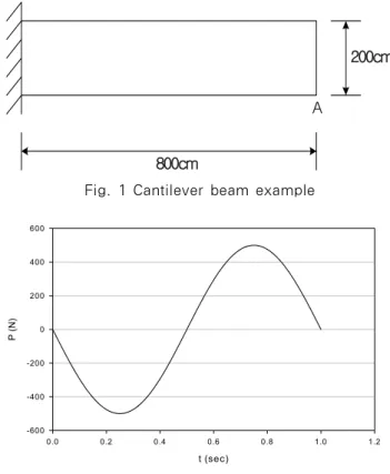
800cm
200cm
A
Fig. 1 Cantilever beam example
t (sec)
0.0 0.2 0.4 0.6 0.8 1.0 1.2
P (N)
-600 -400 -200 0 200 400 600
Fig. 2 Time variation of load P Various means of combining have been studied (de
Las Casas, 1988; Hwang, 1988; Yoon and Jeong, 2005).To obtain an optimal combination of r-method and h-method, first the representative strain values are normalized at each step using the following equations.
× (17)
× (18)
Here, , are the minimum and maximum values of the representative strains, and a, b are constants in each step determined from Eq.
(17) and Eq. (18). These two equations are used to normalize the representative strains to range from 0 to 100.
A dispersion parameter is defined as follows:
(19)
Here, is the average of the normalized repre- sentative strains and is the mode of distribution of the representative strain values. A value for need to be set to combine the r-method and the h-method and a reasonable value is around 20 where if is larger than this value, r-method is used, and in other cases, the h-method is used.
In the h-method, the refinement of the mesh is terminated when the change in the representative strain values is less than 1% or when the element's discretization parameter is less than in Eq. (16).
In the r-method, the refinement of the mesh is termi- nated when the element's discretization parameter is less than in Eq. (16).
3. Case Study
The example considered is a deep cantilever beam shown in Fig. 1 where the dimensions are shown.
The beam is modeled with four node isoparametric quadrilateral elements. The dynamic loading is a lateral concentrated load P where the value is a function of time. The variation of value considered
is given by the following equation:
(20)
The duration of the loading is 1 second as shown in Fig. 2 and the unit for loading is Newton. Since the free vibration response continues after 1 second, the response considered is for 5 seconds. A crude initial mesh formed by four equal elements arranged along the beam axis is used for the investigation.
More appropriate initial mesh increases the efficiency of the algorithm.
The beam is 5cm thick and the material obeys Hooke's law for elasticity with the modulus of elasticity of 210×105N/cm2 and Poisson's ratio of 0.3.
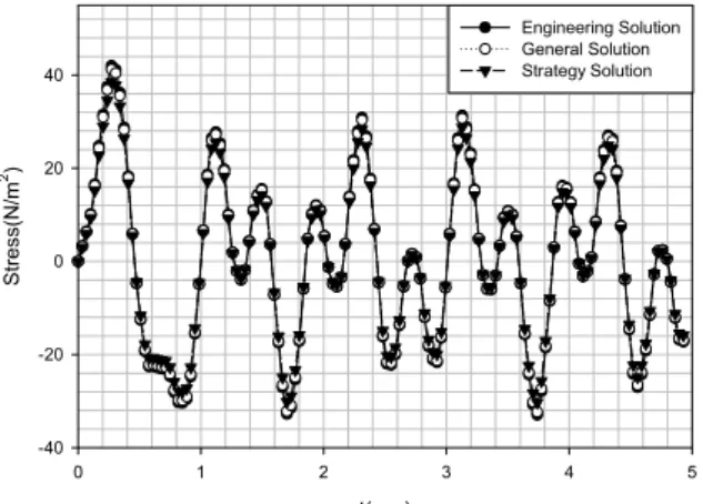
The unit mass is 7.85×10⁻³kg/cm3. The time step selected for analysis is 0.034 seconds yielding 145 steps. For comparison purposes, solutions from a regularly discretized mesh of 1024 elements is termed the engineering solution, the ones from 256 elements is terms the general solution, and the solution from the converged adaptive mesh is termed the strategy solution. Fig. 3, Fig. 4, Fig. 5 and Fig.
t(sec)
0 1 2 3 4 5
Displacement at A(cm)
-0.004 -0.003 -0.002 -0.001 0.000 0.001 0.002 0.003 0.004
Engineering Solution General Solution Strategy Solution
t(sec)
0 1 2 3 4 5
Stress(N/m2)
-40 -20 0 20 40
Engineering Solution General Solution Strategy Solution
Fig. 3 Vertical displacement of the free end Fig. 4 Mid-horizontal normal stress at the fixed end
t(sec)
0 1 2 3 4 5
Stress(N/m2)
-10 -5 0 5 10
15 Engineering Solution
General Solution Strategy Solution
t(sec)
0 1 2 3 4 5
Stress(N/m2)
-10 -5 0 5
10 Engineering Solution
General Solution Strategy Solution
Fig. 5 Mid-vertical normal stress at the fixed end Fig. 6 Mid-shear stress at the free end
Step Method
Maximum.
Representative Strain (%)
Sum of Representative
Strain (%)
Variation of Representative
Strain (%)
0 0.0000297 0.0000659 -
1 h 0.0000057 0.0000456 30.81
2 h 0.0000011 0.0000253 44.53
3 r 0.0000009 0.0000251 0.72
4 r 0.0000008 0.0000251 0.14
5 r 0.0000008 0.0000250 0.16
6 h 0.0000002 0.0000147 41.22
Table 1 Representative strain values for the adaptive scheme
6 show respectively, the comparisons of the vertical displacement of the free end, the mid-horizontal (x directional) normal stress at the fixed end, the mid-vertical (y directional) normal stress at the fixed end, the mid-shear stress at the free end of the engineering, the general, and the strategy solutions.
The figures show close agreement among the three solutions.
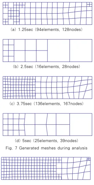
Table 1 shows the representative strain values in the initial steps of the dynamic adaptive mesh where the transitions of the r-method and the h-method are shown. Fig. 7 shows some samples of the generated mesh during the analysis and Fig. 8 shows the mesh during the maximum deflection at the free end which is at 0.275 seconds, where the number of elements is 193 and the number of nodes is 232. Note that at the boundary between fine and coarse mesh, the nodes at the middle of the coarse mesh is slaved to the end nodes for displacement compatibility.
Although the computing efficiency is continuously increasing in general, the enormous amount of computing needed in the time domain finite element dynamic analysis of structures, computing efficiency in every aspect of the algorithm is important in order for the method to be practical (Ladeveze and Oden, 1998;
MacLeod, 2002; Rafiz and Easterbrook, 2005). Table 2 shows the comparative computation times and error
Solution Method
Displacement Error vs Engineering
(%)
Stress Error vs Engineering
(%)
Analysis Time (Reduction vs Engineering in %)
Engineering 0.00 0.00 6hrs 4min 10sec
(0.00)
General 0.72 1.84 8min 14sec
(2.260)
Strategy 3.11 8.03 2min 1sec
(0.553) Table 2 Comparative computation times and error
(a) 1.25sec (94elements, 128nodes)
(b) 2.5sec (16elements, 28nodes)
(c) 3.75sec (136elements, 167nodes)
(d) 5sec (25elements, 39nodes) Fig. 7 Generated meshes during analysis
Fig. 8 Mesh during the maximum deflection at the free end (0.275sec, 193elements, 232nodes)
where it shows reasonable accuracy and extreme computational efficiency of the strategy solution when compared to the engineering solution; only 8.03% error increase at 0.553% computing time.
4. Conclusions
A dynamically adaptive mesh generation scheme for dynamic analyses of structures in time domain is presented. The scheme uses representative strain value from each element computed from the previous time step for estimation of error and an efficient combination of the r-method and the h-method for mesh refinement. Analysis of the application of the proposed scheme to a cantilever beam example shows the following conclusions.
1) The representative strain value for estimation of error gives reasonable relative error. Since the computational requirement is small, the scheme is computationally efficient and successfully achieves the objective of identifying relative errors among the previous elements.
2) An efficient combination scheme combining the traditional r-method and the h-method of is shown to be practical as checks for limiting distortions of elements are incorporated.
The proposed adaptive mesh algorithm is computa- tionally efficient and thus the scheme has potential to be appropriate for real time computations of large complex structures under erratic time dependent loads such as earthquakes and turbulent winds, problems important in maintenance of structures and structural hazard mitigation. Some aspects of the scheme still need to be improved, one of which is the appropriate selection of the initial mesh that starts the algorithm.
Acknowledgements
This work was supported by 2008 Hongik University Research Fund.
References
Bathe, K.J., Wilson, E.L. (1976) Numerical Methods in Finite Element Analysis, Prentice Hall, Englewood Cliffs.
Belytschko, T. (1974) Transient Analysis, Structural Mechanics, Computer Programs, Surveys, Assessments,
and Availability, Edited by Pilkey, W., Saczalski, K.
and Schaeffer, H. University of Virginia Press, Charlottesville, Virginia, pp.255~276.
Belytschko, T., Hughes, J.R., Bathe, K.J. (1996) Finite Element Procedures, Prentice-Hall, Englewood Cliffs.
Choi, C., Jung, H. (1998) Adaptive Mesh Generation for Dynamic Finite element Analysis, J. Korean Soc.
of Civil Eng.(in Korean), 18(Ⅰ-2), pp.203~220.
Choi, C.K., Yu, W.J. (1998) Adaptive Finite Element Wind Analysis with Mesh Refinement and Recovery (in Korean), Wind and Structures, 1, pp.111~125.
Cook, R.D., Malkus, D.S., Plesha, M.E. (1989) Concepts and Applications of Finite Element Analysis, 3rd Ed. John Wiley & Sons, New York.
de Las Casas, E.B. (1988) R-H Mesh Improvement Algorithms for the Finite Element Method, Ph.D.
Dissertation, Purdue University, West Lafayette.
Heesom, D., Mahdjoubi, L. (2001) Effect of Grid Resolution and Terrain Characteristics on Data from DTM, J. Comp. in Civil Eng., ASCE, 15(2), pp.137~143.
Hwang, S.W. (1988) A Study on the r-h Method in the Finite Element Method, Master's Thesis(in Korean), Inha University, Inchon.
Jeong, Y.C., Yoon, C. (2003) Representative Strain Value Based Adaptive Mesh Generation for Plane Stress, Hongik J. Science and Tech., 7, pp.71~86.
Jeong, Y.C., Yoon, C., Hong, S. (2003) Adaptive Mesh Generation Scheme for Planar Problems using Representative Strain Values for Error(in Korean), Proc., Korean Soc. Comp. Structural Eng., 16 (2-31), pp.403~409.
Ladeveze, P., Oden, J.T., Editors. (1998) Advances in Adaptive Computational Methods in Mechanics Studies in Applied Mechanics, 47, Elsevier, Oxford.
MacLeod, I.A. (2002) The Education of Structural Analyst, Proc., Asranet Symp., Asranet, Dept. of Naval Architecture and Marine Eng., Univ. of Glasgow and Strathclyde, London.
McFee, S., Giannacopoulos, D. (2001) Optimal Discretizations in Adaptive Finite Element Elect- romagnetics, Int. J. Numer. Meth. Eng., 52(9), pp.939~978.
Newmark, N.M. (1959) A Method of Computation for Structural Dynamics, J. Eng. Mech. Division, American Society of Civil Engineers, 85(EM3), pp.67~94.
Ohnimus, S., Stein, E., Walhorn, E. (2001) Local Error Estimates of FEM for Displacements and Stresses in Linear Elasticity by Solving Local Neumann Problems, Int. J. Numer. Meth. Eng., 52(7), pp.727~746.
Rafiq, M.Y., Easterbrook, D.J. (2005) Using the Computer to Develop a Better Understanding in Teaching Structural Engineering Behavior to Under- graduates, J. Comp. in Civil Eng., 19(1), pp.34~44.
Reddy, J.N. (1993) An Introduction to the Finite Element Method, 2nd Ed., McGraw-Hill, New York.
Stampfle, M., Hunt, K.J., Kalkkuhl, J. (2001) Efficient Simulation of Parameter-Dependent Vehicle Dynamics, Int. J. Numer. Meth. Eng., 52(11), pp.1273~1299.
Yoon, C. (2005) Adaptive Mesh Generation for Dynamic Finite Element Analysis(in Korean), J.
Korean Soc. Civil Eng., 25(6A), pp.989~998.
Yoon, C. (2009) Computer Aided Teaching of Structural Engineering Using Adaptive Schemes in the Finite Element Method, J. Korean Soc. Hazard Mitigation., 9(1), pp.9~13.
Zhu, J.Z., Zienkiewicz, O.C., Hinton, E., Wu, J.
(1991) A New Approach to the Development of Automatic Quadrilateral Mesh Generation, Int. J.
Numer. Meth. Eng., 32, pp.849~866.
Zienkiewicz, O.C., Taylor, R.L., Zhu, J.Z. (2005) The Finite Element Method: Its Basis and Funda- mentals, 6th Ed. Elsevier Butterworth-Heinemann, Oxford.
Zienkiewcz, O.C., Zhu, J.Z. (1987) A Simple Error Estimator and Adaptive Procedure for Practical Engineering Analysis, Int. J. Numer. Meth. Eng., 24, pp.337~357.
논문접수일 2010년 10월 30일
논문심사일 2010년 11월 4일
게재확정일 2010년 11월 29일