Ⅰ. Introduction
Glioma is the most common type of brain tumor arising from glial cells. Gliomas may have different degrees of aggressiveness, variable prognosis, and several heterogeneous histological sub-regions that are described by varying intensity profiles across different Magnetic Resonance Imaging (MRI) modalities which reflect diverse tumor biological properties [1]. Accurate segmentation and measurement of the different tumor sub-regions is critical for monitoring progression, surgery or radiotherapy planning, and follow-up studies.
However, the distinction between tumors and normal tissue is difficult to discern as the tumor’s borders are often fuzzy, and there is a high variability in shape, location, and extent across patients. Despite recent advances in automated algorithms for brain tumor segmentation in multimodal MRI scans, the problem is still a challenging task in medical imaging analysis [2][3][4].
Manual annotation of such data is a difficult and time consuming task. Since experts can only view a single 2D slice of a 3D scan at a time. It’s also quite inefficient since neighboring slices contain
* corresponding author
mostly the same information. Although development and implementation of automated segmentation algorithms is a challenging task, it can greatly benefit experts in the field. Furthermore, it has great potential to aid in better diagnoses, surgical planning, and treatment assessment of brain tumors [2].
In this paper, we demonstrate the capabilities of a deep neural network that learns to automatically segment tumors in 3D MRI scans using 2018 BraTS dataset to train and validate the proposed algorithm. All BraTS multimodal scans describe a) native (T1) and b) post-contrast T1-weighted (T1Gd), c) T2-weighted (T2), and d) T2 Fluid Attenuated Inversion Recovery (FLAIR) volumes, and were acquired with different clinical protocols and various scanners from multiple (n=19) institutions.
All the imaging datasets have been segmented manually by one to four raters, following the same annotation protocol, and their annotations were approved by experienced neuro-radiologists.
Annotations comprise the GD-enhancing tumor, the peritumoral edema, and the necrotic and non-enhancing tumor core. [1]
Our proposed CNN is based on U-net inspired architecture described in [5], however the
Automatic Volumetric Brain Tumor Segmentation using Convolutional Neural Networks
Vladyslav Yavorskyi · Sanghoon Sull* Korea University
E-mail : [email protected] / [email protected]
ABSTRACT
Convolutional Neural Networks (CNNs) have recently been gaining popularity in the medical image analysis field because of their image segmentation capabilities. In this paper, we present a CNN that performs automated brain tumor segmentations of sparsely annotated 3D Magnetic Resonance Imaging (MRI) scans. Our CNN is based on 3D U-net architecture, and it includes separate Dilated and Depth-wise Convolutions. It is fully-trained on the BraTS 2018 data set, and it produces more accurate results even when compared to the winners of the BraTS 2017 competition despite having a significantly smaller amount of parameters.
Keyword
CNNs, 3D U-Net, Medical Image Segmentation, Brain Tumor Segmentation
432
한국정보통신학회 2019년 춘계 종합학술대회 논문집
implementation of Dilated [9] and Depth-wise separate convolutions [10] allows us to get even
better results with almost the half of the parameters of the original network.
Ⅱ. Methods
Data preprocessing: MR scans often display intensity non-uniformities due to variations in the magnetic field. So, one part of an image might appear lighter or darker when visualized solely because of variations in the magnetic field. The map of these variations is called the bias field. The bias field can cause problems for a classifier as the variations in signal intensity are not due to any anatomical differences. We use Advanced Normalization Tools (ANTs) N4 Bias Field Correction in an attempt to correct the bias field by extracting it from the image. We also use a number of data augmentation techniques in data preprocessing.
Network architecture is based on [5] U-Net inspired architecture, shown in Figure 1. The network is designed to process large 3D input blocks of 128x128x128 voxels.
Just like the U-Net architecture, our CNN comprises a context aggregation pathway that encodes increasingly abstract representations of the input as we progress deeper into the network. This is followed by a localization pathway that
recombines these representations with shallower features to precisely localize the structures of
interest. We refer to the vertical depth (the depth in the U shape) as level, with higher levels being lower spatial resolution, but higher dimensional feature representations.
The activations in the context pathway are computed by context modules. Each context module is comprised of two Depth-wise separable convolution blocks with dilated convolutions, whereas dilation rate increases for deeper layers, in order to increase the receptive field of the network and a dropout layer in between. Context modules are connected by 3x3x3 convolutions with input stride 2 to reduce the resolution of the feature maps, and allow for more features while descending down the aggregation pathway.
As stated previously, the localization pathway is designed to take features from lower levels of the network that encode contextual information at low spatial resolution, and then transfer that information to a higher spatial resolution. We achieve this through up-sampling the low-resolution feature maps by means of a simple upscale that repeats the feature voxels twice in each spatial dimension followed by a 3x3x3 convolution that halves the number of feature maps.
We then recombine the up-sampled features with the features from the corresponding level of the context aggregation pathway via concatenation.
Following the concatenation, a localization module recombines these features together and further reduces the number of feature maps. This is critical Figure 1. Network Architecture
433
한국정보통신학회 2019년 춘계 종합학술대회 논문집
for reducing memory consumption. A localization module consists of a 3x3x3 dilated convolution with a dilation rate decreasing for the shallow layers followed by a 1x1x1 convolution that halves the number of feature maps.
We employ deep supervision in the localization pathway by integrating segmentation layers at different levels of the network, and combining them via element-wise summation to form the final network output. Throughout the network we use leaky ReLU nonlinearities with a negative slope of 10−2 for all feature map computing convolutions.
We furthermore replace the traditional batch with instance normalization [7] since we found that the stochasticity induced by our small batch sizes may destabilize batch normalization.[5]
The addition of depth-wise separable convolutions and dilated convolutions with dilation rates that vary for layers of different depths to the context and localization modules helps us to increase accuracy and greatly reduce the number of parameters needed for the network.
Dice loss function: In MRI scans that we are processing, anatomy of interest occupies only a very small region of the scan. This often causes the learning process to get trapped in local minima of the loss function yielding a network whose predictions are strongly biased towards background.
As a result, the foreground region is often missing or only partially detected. In this work we use an objective function based on dice coefficient, which is a quantity ranging between 0 and 1 which we aim to maximize. The dice coefficient D between two binary volumes can be written as
where the sums run over the N voxels of the predicted binary segmentation volume and the ground truth binary volume . This formulation of Dice can be differentiated by yielding the gradient
computed with respect to the j-th voxel of the prediction. Using this formulation, we can achieve the right balance between foreground and background voxels. [6]
Ⅲ. Results
We trained our network from the scratch on BraTS 2018 dataset. In Table 1, we compare the performance of our algorithm to the [5] and other state-of-the-art algorithms in the BraTS competition.
Our method compares favorably to other state-of-the-art neural networks while having an almost 50% reduction in parameters, due to the use of the depth-wise separable convolutions. There is no native implementation for the 3D depth-wise separable convolutions in keras library, deep learning library that we used in this paper.
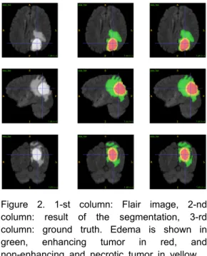
Therefore, we had to implement our own which resulted in our network having 3,757,945 parameters, or only 45% compared to [5] with 8,269,331 parameters. Results of automatic segmentation are shown in Figure 2.
Figure 2. 1-st column: Flair image, 2-nd column: result of the segmentation, 3-rd column: ground truth. Edema is shown in green, enhancing tumor in red, and non-enhancing and necrotic tumor in yellow.
Table 1. Dice scores of validation set for winners of the BraTs 2017 competition and our proposed model.
434
한국정보통신학회 2019년 춘계 종합학술대회 논문집
Ⅳ. Conclusion
In this paper, we present a deep convolutional neural network architecture, trained on the BraTS 2018 dataset concerning the MRI scans of brain tumor patients that can perform an automatic segmentation of these images. With small changes, the proposed network can be trained on any other sparsely annotated MRI images, and thus can be applied to many other biomedical volumetric segmentation tasks. Our network demonstrates satisfactory results - an average dice score of 0.846 at this point. We are planning to upgrade the architecture to a cascaded network in the future to take advantage of the gliomas cascaded structure.
Other improvements like increasing batch size or the depth of the network can be made to ensure the network can be trained on more powerful machines with multiple GPUs.
References
[1] Menze BH, et al. "The Multimodal Brain Tumor Image Segmentation Benchmark (BRATS)", IEEE Transactions on Medical Imaging 34(10), 1993-2024 (2015) DOI:
10.1109/TMI.2014.2377694
[2] Bakas S, et al. "Advancing The Cancer Genome Atlas glioma MRI collections with expert segmentation labels and radiomic features", Nature Scientific Data, 4:170117 (2017) DOI:
10.1038/sdata.2017.117
[3] Bakas S, et al. "Segmentation Labels and Radiomic Features for the Pre-operative Scans of the TCGA-GBM collection", The Cancer Imaging Archive, 2017. DOI:
10.7937/K9/TCIA.2017.KLXWJJ1Q
[4] Bakas S, et al. "Segmentation Labels and Radiomic Features for the Pre-operative Scans of the TCGA-LGG collection", The Cancer Imaging Archive, 2017. DOI:
10.7937/K9/TCIA.2017.GJQ7R0EF
[5] Isensee, F., Kickingereder, P., Wick, W., Bendszus, M., Maier-Hein, K.H.: Brain Tumor Segmentation and Radiomics Survival Prediction:
Contribution to the BRATS 2017 Challenge.
arXiv:1802.10508 [cs]. (2018)
[6] F. Milletari, N. Navab and S. Ahmadi, "V-Net:
Fully Convolutional Neural Networks for Volumetric Medical Image Segmentation,"
Fourth International Conference on 3D Vision (3DV), Stanford, CA, USA, 2016, pp. 565-571.
(2016)
[7] D. Ulyanov, A. Vedaldi, and V. Lempitsky,
“Instance normalization: The missing ingredient for fast stylization,” arXiv preprint arXiv:1607.08022, 2016.
[8] G. Wang, W. Li, S. Ourselin, and T.
Vercauteren, “Automatic brain tumor segmentation using cascaded anisotropic convolutional neural networks,” in Brainle-sion:
Glioma, Multiple Sclerosis, Stroke and Traumatic Brain Injuries, A. Crimi, S. Bakas, H. Kuijf, B. Menze, and M. Reyes, Eds. Cham:
Springer International Publishing, 2018, pp. 178–
190.
[9] Fisher Yu, Vladlen Koltun, et al. "Multi-Scale Context Aggregation by Dilated Convolutions", ICLR 2016, arXiv:1511.07122
[10] François Chollet, "Xception: Deep Learning with Depthwise Separable Convolutions", arXiv:1610.02357, 2016
435