Semantic Correspondence of Database Schema from Heterogeneous Databases using Self-Organizing Map
Menchita F. Dumlao*, Byung-Joo Oh
★Abstract
This paper provides a framework for semantic correspondence of heterogeneous databases using self- organizing map. It solves the problem of overlapping between different databases due to their different schemas. Clustering technique using self-organizing maps (SOM) is tested and evaluated to assess its performance when using different kinds of data. Preprocessing of database is performed prior to clustering using edit distance algorithm, principal component analysis (PCA), and normalization function to identify the features necessary for clustering.
Keyword: Semantic integration, heterogeneous databases, semantic correspondence, clustering, data pre-processing, self-organizing maps.
I. Introduction
Semantic integration is an active area of research for heterogeneous databases. Inter- operability between different databases is necessary for sharing the resources which are different in format and platforms. Semantics focuses on the meaning of data. Semantic correspondence deals with the similarity of schema and instance in a database. In database application, different databases are designed with different formats, but contains the same meaning. Most of the time, the attributes of heterogeneous databases overlap
* College of Engineering, Hannam University
★Professor of Electronics Engineering E-mail:[email protected]
※ Acknowledgement
This work was supported by Research Grant(2008) from Hannam University and the Security Engineering Research Center, granted by the Korea Ministry of Knowledge Economy.
because they are represented differently in terms of their names, data patterns, schema specification, document similarity and usage pattern.
Nowadays, the demand for integrating business systems varies from file sharing systems, information systems, database systems and enterprise systems. Data from one source is often needed by another system which generally requires the integration of data from one department to another department. For example, business merging often needs to integrate customer records of two businesses. In most cases, records are identical but the structure to which data are stored, presented and accessed are different.
However, the semantics of a database schema can be used to identify the pattern of similarity between databases. We focus on the similarity of attributes in terms of their semantics which means two different databases may have the same records even though they have different structures.
Many researchers have tried to solved this problem like the pre-integration and comparison of schemas which is done to conform, merge, map and restructure schemas
(217)
[1]. Schema translation, inter-schema relationship, integrated schema generation and schema mapping generation were done to study the similarity between schema structure [2] . Schema analysis, class integration, and schema restructuring [3], B-schema translation, T-schema creation, and comparison of B-schema and T-schema [4]
were proposed to solve the problem in schema integration. Zhao uses SOM to detect schema correspondence of heterogeneous data sources [5]. SOM was tested using e-catalog database, airline database and property management database. SOM was proven to be an effective tool for semantic correspondence, but it was tested with clean data. In our study, we used a more complex database, the customer database, to test the robustness of SOM in clustering a different kind of data.
In section II we discussed the overview of clustering. Section III describes our new set of data which is the customer database. In 3.1 to 3.2 we describe the nature of features and the techniques of extracting features from raw database schema to feature vectors which includes, edit distance, summary of statistics and PCA. Section 3.3 is focused on clustering using SOM, section IV discussed evaluation of results and section V deals with the conclusion of our study.
II. Overview of Clustering
Cluster analysis techniques group objects from some problem domain, into unknown groups called clusters, such that objects within the same clusters are similar to each other, while objects across clusters are dissimilar to each other. The objects to be clustered are represented as vectors of features, or variables. Principal component analysis or factor analysis can be performed prior to clustering to reduce the dimensionality of input vectors[15].
We use cluster analysis technique to determine the correspondence between schemas. The schema is composed of the attributes of the database which describes how data is defined in the database. The characteristics of the attributes (i.e., fields)
were identified to determine the features needed for the clustering technique. There are two main features used in this study, naming similarity and data pattern. Naming similarity is one of the features used in clustering technique. Edit distance function is used to get the value for naming similarity. Two attributes are compared using edit distance to be able to produce a value range from 0..1.
Data patterns is another feature extracted from database. The summary of statistics of each attribute in the database are computed using the functions: average, count of missing values, count of distinct values, average of length of values, standard deviation of length of values, maximum, statistics on percentage of digits in the attribute values, statistics on the percentage of letters in the attribute values.
The accumulated values from naming similarity and data patterns were combined and then preprocessed using PCA. The result of summary of statistics are normalized into range 0 to 1 before it is inputted to SOM.
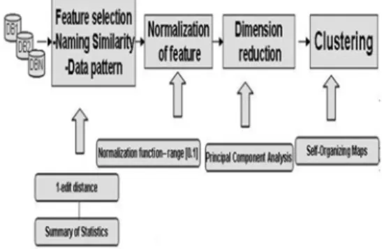
Figure 3.Process and Techniques for Semantic Correspondence
III. Clustering Approach for Semantic Correspondence of
Database Schema.
We proposed clustering of schema elements using SOM. We used two customer databases that we purposely created to test SOM. It has different number of tuples, and has different number of attributes found in each databases. The names given to each attributes are intended to be named differently
(218)
to be able to test the performance of SOM in clustering opaque attributes with exactly the same instances. We extracted the customer list of Neurodimension Company and assigned fictitious attributes to create a customer database for Neurodimension. WE also extracted the customer list of the MySQL Company and create a database the same way that we did as that with the Neurodimension database. Figure 1 and figure 2 shows some attributes and instance of our test database.
Figure 1. Some parts of Neurodimension Database.
Figure 2. Some parts of Mysql Company Database.
We intend to integrate the attributes of Neurodimension database and Mysql database using SOM. Figure 3 illustrates our approach in clustering database schema.
3.1 Feature Extraction of Database Schema for Cluster Analysis
The input to SOM are real numbers that range from 0..1. We intend to determine the similarity of two or more heterogeneous database by using clustering technique through SOM. We extract features needed for clustering by identifying the most significant characteristics of database that describes their relationships. These are the semantic features about schema elements namely, naming similarity, document similarity, schema specification[10] [11] [12], data pattern, usage pattern, business rules and integrity constraints, user’s mind and business process[7]. We used naming similarity and data pattern to extract the features of customer database. Figure 4 shows some values for naming similarity and figure 5 shows some of the features from data pattern.
3.1.1 Naming Similarity
These are names that describes the structure of databases. Database tables and attributes should be named in accordance to the meaning that it reflect. Many problems in naming schema elements caused difficulties in identifying the similarity of databases. Their semantics cannot be defined because of some technical issues:
(1)Some attributes have opaque names that their meanings do not describe the data or record that it represent. (2) Schema element names usually cannot completely capture the semantics of elements. (3) In some regions where pictographic languages are officially used, pronunciation notation are used to name database objects, thus the pronunciation may mean many totally different things[7].
We extracted 45 features using naming similarity, where each attribute from the two customer database are compared using 1-edit distance[8] algorithm to compute for the similarity of two attributes.
A commonly used bottom-up dynamic programming for computing edit distance involves the use of an (n+1) x (m+1) matrix[9]. Where n and m are the lengths of two strings. Figure 4 shows some of the values for naming similarity using 1-edit distance.
(219)
3.1.2 Data Patterns
The pattern of records in a database are the statistics of actual data samples that can be used for cluster analysis. Pattern of value include: the length of a value, the percentage of digits within a string, and the percentage of special characters within a string. Pattern of an attribute includes statistics (central tendency and variability) of the pattern of its values, the ratio of the number of distinct values to the number of records, and the percentage of missing and non-missing values. The problem with data pattern is that they are often correlated with structures than with semantics.
We extracted 14 data patterns by computing the summary of statistics of the instances or records of customer database.
We compute for the count of missing values, count of distinct values, average length, standard deviation of length, min and max of length, average number of digits and average number of characters, min and max of percentage of digits in the records of each attribute, average of percentage of digits in the record of each attribute, standard deviation of the percentage of digits in the record of each attribute, min and max of percentage of character in the records of each attribute, average of percentage of character in the record of each attribute, standard deviation of the percentage of character in the record of each attribute.
After computing the summary of statistics, the values are normalized using the normalization function,
( ) ( min) /(max min)
f x = x− −
(1) where, x is the value to be normalized, and min and max are minimum and maximum of each feature. Figure 5 shows some of the results extracted for data pattern.
Figure 4. Naming similarity features using 1- edit distance.
Figure 5. Data pattern using summary of statistics.
3.2 Principal Component Analysis for Dimensionality
Reduction of Features
After extracting the features of our dataset, we perform PCA to reduce the dimension of data that will be used as input to our clustering algorithm, the SOM. PCA is the way of identifying patterns in data, and expressing the data in such a way as to highlight their similarities and differences.
Since patterns in high dimensional data can be hard to find, PCA is a powerful tool for analysis. PCA compression is possible without much loss of information[13].
The algorithm of PCA is summarized in the following steps: (1) subtract the mean, (2) calculate the covariance matrix: The definition for the covariance matrix for a set of data with n dimensions is:
, , . ,
( ( , cov(
nxn
i j i j i j
C = C C = Ci j= Dim Dim ))
(220)
where is a matrix with n rows and n columns, and
Cnxn
Dimx is the xth dimension. If you have an _ -dimensional data set, then the matrix has _ rows and columns (so is square) and each entry in the matrix is the result of calculating the covariance between two separate dimensions. (3) calculate eigenvectors and eigenvalues of co-variance matrix, (4) choosing component and forming a feature vector, (5) deriving the new dataset, and (6) getting the old data back[14].
We used SPSS Clementine’s PCA modeling to reduce the dimension of our feature arriving at 14 factors from the 59 features extracted using naming similarity and data pattern. The PCA model that uses correlation matrix between input fields are identified, and the maximum iterations for convergence is set to 25. The extraction factors was set to eigenvalues over 1.0. After PCA, our dataset was reduced from 45 row by 59 columns to 45 rows by 14 columns. The reduced feature is our input to SOM.
3.3 Clustering Using Self-Organizing Maps.
Self-organizing maps are unsupervised learning methods that generally fall under neural network technique that employ competitive learning algorithm(CLA). Given a set of cluster representatives pairs, wj , j=1…m (m is the number of clusters), the idea behind CLA is to move each of these representatives to the regions of the vector space that are dense in vectors of x.
The term “competitive” arises form the fact that when an input pattern x is presented, each wj equation always compete with each other. The winner, is the wj that lies closer to x, which is then updated so as to move toward x, while losers either remain stationary or are used x slowly. For a detailed exposition of the Generalized CL Section (GCLS) see [6].
An important component of GCLS is the update of the cluster representatives, following distance evaluation between input pattern and representative wj, in SOM, this is expanded as:
( ) ( ) ( 1) ( )( ( 1))
( ) ,
( 1)
k j
r k
K
k
if w t Q t w t n t x w t
w t w t otherwise
∈
⎧ − + − −
=⎨⎩ −
(2)
Note in the above equation that, not only the single close to ‘x’ is updated but rather whole neighborhood but the 2
wi
j( )
Q t nd term
in the last line denotes that such an update is also dependent on the distance between x andwk∈Q tj( ) aside from the learning rate
( )t
η
.We perform clustering using SOM in SPSS Clementine. We use 45 by 14 matrix of features accumulated after PCA. We use expert training methods to specify the topology of kohonen net and the learning rates used for training. The topology of a Kohonen network in Clementine is always a 2 dimensional rectangular grid. We set our map to a 6 by 6 grid, and the learning rate to exponential.
Kohonen net training is split into two phases. Phase 1 is a rough estimation phase, used to capture the gross patterns in the data.
Phase 2 is a tuning phase, used to adjust the map to model the finer features of the data.
For each phase, there are three parameters.
We set the starting size (radius) of the neighborhood into 2, to determine the number of nearby units that gets updated along with the winning unit during training. During phase 1, the neighborhood size starts at phase 1 neighborhood and decreases to Phase 2 Neighborhood +1. During Phase 2, neighborhood size starts at phase 2 neighborhood and decreases to 1.0. Phase 1 Neighborhood should be larger than phase 2 neighborhood[15].
We perform clustering using SPSS for customer database and used the combination of parameters that includes: (1)Phase 1:
neighborhood =15, initial eta=0.3, cycles=50;
(2) Phase 2: neighborhood=1, eta=0.1, cycles=150.
During phase1, eta starts at phase 1 initial eta and decreases to phase 2 initial eta. During phase 2, eta starts at phase 2 initial eta and decreases to 0. Phase 1 initial eta should be larger that phase 2 initial eta.
(221)
During training, each grid square competes with all the others to ‘win’ each record. “Strong” nodes will win more records and “weak” nodes may win no records at all.
As the grid squares competes, the training regime ‘settles’ the network onto a stable classification, capturing as much of the information in the training records as possible.
We use another database, the E-catalog database to test our approach. We use the dataset that was used in [7]. We preprocess the e-catalog database, normalize the features in range 0,1 and then perform PCA. We have 30 rows by 44 columns of features, and reduce it to 30 by 10 columns after PCA. We perform clustering using SPSS and used the combination of parameters that includes:
(1)Phase 1: neighborhood =2, initial eta=0.3, cycles=20; (2) Phase 2: neighborhood=1, eta=0.1, cycles=150.
IV. Discussion and Evaluation of Results
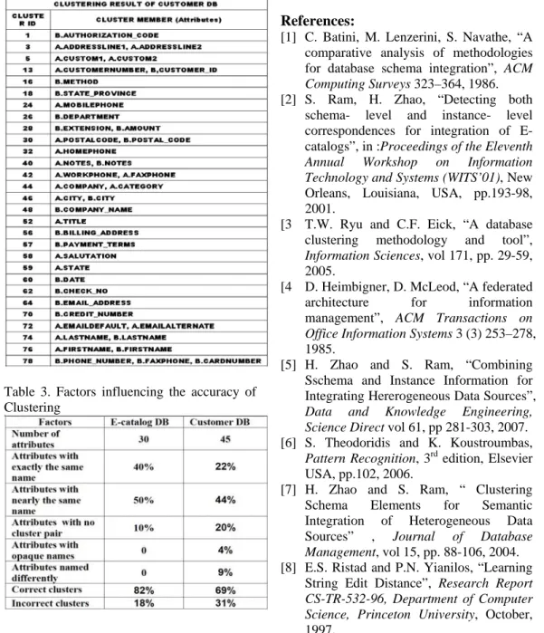
We have 20 correct clusters out of 28 clusters of attributes for customer database after performing SOM. Clusters with cluster id numbers 18,24,28,32,44,48,52,56,59 are considered incorrect clusters because they are grouped with wrong cluster member. For the e-catalog database, we have 9 correct clusters out of 11. Table 1 summarizes the result of clustering for e-catalog database. There are 9 correct clusters and 2 incorrect clusters.
Clusters with cluster id 2 and 13 are considered incorrect clusters. A.MONTH should be pair with B.MONTH and A.SERIES should have no pair. Table 2 shows the results of clustering for customer database.
We use two types of databases to test the accuracy of our approach. We perform the same procedure to both customer database and e-catalog database but the clustering of attributes in the e-catalog database resulted into more accurate clusters.
We compared the complexity of each databases and we identify some factors that
influenced the results of our experiments. Our observation is summarized in table 3.
Table 1. Result of Clustering for E-catalog
We observed that the complexity of database affects the accuracy of clustering.
The accuracy of clustering using e-catalog is higher at 82% than customer database at 69%.
In the customer database, 22% of attributes are named exactly, compared to the e-catalog database with 40% exact names. The rate of attributes which are named differently is larger in the customer database at 9%
compared to e-catalog database at 0%.
Customer database has 4% opaque names while the e-catalog database has none. Our observation shows that naming similarity significantly affects the clustering performance of our SOM.
V. Conclusion
We performed semantic integration using SOM and we got 69-82% correctness and 18- 31% incorrect clusters for e-catalog and customer database, respectively. The performance of self-organizing maps as an effective tool for cluster analysis varies from one application to another with respect to the complexity of input features, parameters, kind of input features for clustering, and the level of clustering that we want to produce. SOM has the ability to determine the similarity of inputs based on the amount of features that was inputted to the network. The learning rate of SOM, neighborhood, cycle and training time may be able to detect similarity, but it
(222)
does not guarantee the accuracy of clusters.
We should also consider the complexity of our input features, the expected clusters that we want to meet, and the process of extracting the features for clustering.
Table 2. Result of Clustering for Customer Database
Table 3. Factors influencing the accuracy of Clustering
The larger number of naming similarity features compared to the number of data pattern features affects the clustering performance of SOM. In principle, our clustering should represent the similarity of records in database rather than show the similarity of attribute names. In this sense, the number of correct clusters varies significantly with the complexity of database.
References:
[1] C. Batini, M. Lenzerini, S. Navathe, “A comparative analysis of methodologies for database schema integration”, ACM Computing Surveys 323–364, 1986.
[2] S. Ram, H. Zhao, “Detecting both schema- level and instance- level correspondences for integration of E- catalogs”, in :Proceedings of the Eleventh Annual Workshop on Information Technology and Systems (WITS’01), New Orleans, Louisiana, USA, pp.193-98, 2001.
[3 T.W. Ryu and C.F. Eick, “A database clustering methodology and tool”, Information Sciences, vol 171, pp. 29-59, 2005.
[4 D. Heimbigner, D. McLeod, “A federated architecture for information management”, ACM Transactions on Office Information Systems 3 (3) 253–278, 1985.
[5] H. Zhao and S. Ram, “Combining Sschema and Instance Information for Integrating Hererogeneous Data Sources”, Data and Knowledge Engineering, Science Direct vol 61, pp 281-303, 2007.
[6] S. Theodoridis and K. Koustroumbas, Pattern Recognition, 3rd edition, Elsevier USA, pp.102, 2006.
[7] H. Zhao and S. Ram, “ Clustering Schema Elements for Semantic Integration of Heterogeneous Data Sources” , Journal of Database Management, vol 15, pp. 88-106, 2004.
[8] E.S. Ristad and P.N. Yianilos, “Learning String Edit Distance”, Research Report CS-TR-532-96, Department of Computer Science, Princeton University, October, 1997.
(223)
[9] P. Hall and G. Dowling, “Approximate String
Matching”, Computing Surveys 12-4 pp. 381-402,
1980.
[10] E. Ellmer, C. Huemer, D.Merkl, G.
Pernul, “Automatic Classification of semantic concepts in view specifications”, in Database and Expert Systems Applications, Proceedings of 7th International Conference, DEXA ’96, pp.824-833, 1996.
[11] W.S. Li and C. Clifton, “SEMINT: A tool for identifying attributer correspondence in heterogeneous databases using neural networks”, Data and Knowledge Engineering, Elsevier, vol 33, pp. 49-84, 2000.
[12] U. Srinivasan , A.H.H. Ngu,., & T.
Gedeon, “Managing heterogeneous information systems through discovery and retrieval of generic concepts”, Journal of American Society for Information Science, 51(8), 707-723, 2000.
[13] J. Shlens, “A Tutorial on Principal Component Analysis”, March, 2003.
[14] L. I. Smith, “A Tutorial on Principal Component
Analysis”, February, 2002.
[15] A.A. Afifi & V. Clark, Computer Aided Multivariate Analysis (3rd ed.), New York: Chapman & Hall, 1996.
[16] Clementine Reference Manual Version 5, Integral
Solutions Limited, July 11, 1995.
BIOGRAPH
MMenchita F. Dumlao
1997. BSICS Lyceum of Batangas, Philippines.
2003. M.S.
Information Technology, Hannam University
2005. ~ Present, Graduate Student, Hannam University.
Interest Area : Data Integration, Database development, System analysis and design, Data mining.
Oh, Byung-Joo
1976. B.S.
Electronic
Engineering, Busan National University, 1983. M.S.
Electrical &
Computer Engineering, University of New Mexico.
1988. Ph.D, Electrical & Computer Engineering, University of New Mexico.
1992. 3. ~ Present, Professor in Electronic Engineering, Hannam University.
Interest Area : Adaptive control, Neural network, Fuzzy logic, Robot control and vision, Face detection and recognition.
(224)