A Finite Mixture Model for Gene Expression and Methylation Pro les in a Bayesian Framewor

A Finite Mixture Model for Gene Expression and Methylation Profiles in a Bayesian Framework

Jaesik Jeong ¹

1 Department of Biostatistics, Indiana University (Received March 2011; accepted June 2011)

Abstract

The pattern of methylation draws significant attention from cancer researchers because it is believed that DNA methylation and gene expression have a causal relationship. As the interest in the role of methylation patterns in cancer studies (especially drug resistant cancers) increases, many studies have been done inves- tigating the association between gene expression and methylation. However, a model-based approach is still in urgent need. We developed a finite mixture model in the Bayesian framework to find a possible relation- ship between gene expression and methylation. For inference, we employ Expectation-Maximization(EM) algorithm to deal with latent (unobserved) variable, producing estimates of parameters in the model. Then we validated our model through simulation study and then applied the method to real data: wild type and hydroxytamoxifen(OHT) resistant MCF7 breast cancer cell lines.

Keywords: Expectation-Maximization, hierarchical statistical model, latent variable, methylation, mix- ture model.

1. Introduction

Epigenetic events (that include DNA methylation) are involved in complex processes of biological interactions that results in the regulation of gene expression (Herman, 1999; Hinshelwood and Clark, 2008; Jeong et al., 2010). DNA methylation is the process that add a methyl group to the 5 position of the cytosine pyrimidine ring, that can be inherited from cell divisions. In mammals, DNA methylation is a crucial part of normal organismal development and cellular differentiation and stably alters the gene expression pattern in cells. In addition, DNA methylation plays a key role in the development of almost all types of cancer (Baylin and Herman, 2000; Bird, 2002; Herman and Baylin, 2003; Dwivedi et al., 2003).

In the clinical setting, drug resistance is a critical issue for cancer treatment. Sometimes drug resistance happens from the beginning of treatment. However, some people do respond first and stop responding after a course of treatment of the same drug that is known as acquired drug resistance.

Reasons for such resistance possibly result from epigenetic events such as DNA methylation and chromatin modification. Especially, epigenetic alteration such as DNA methylation plays a key role in acquired drug resistance (Jones and Laird, 1999; Jones and Baylin, 2007).

1 Post-doctor, Department of Biostatistics, Indiana University, 410 West 10th Street, Suite 3000, Indianapo-

lis, IN 46202, USA. E-mail: [email protected]

As the interest in the role of methylation pattern in cancer study increases, many studies have investigated the association between gene expression and methylation (Ahuja et al., 1997; Muller et al., 2001; Esteller et al., 1999; Hui et al., 2000; Wang et al., 2009). In a classic approach, fold change is used for status call and χ ² test (Fisher’s exact test for small sample) is used to test for association (Ahuja et al., 1997; Muller et al., 2001; Hui et al., 2000). Such methods provide a kind of global view (category-specific) on the interplay between gene expression and methylation. However, there is increasing evidence that such association is gene-specific. Model-based approaches (especially an empirical Bayes model) have been developed to illustrate the evidence of a local view (gene-specific) other than a global view (Jeong et al., 2010).

A hierarchical statistical model in the Bayesian framework (hierarchical Bayes model) was developed by Jeong et al. (2010) and George (1985). They assume normality on log-transformed fold change and specify normal prior on the mean vector. Inference is based on the posterior distribution of the mean vector of each gene. The estimated prior covariance provides a global view and the covariance estimate from the posterior distribution of each gene gives a local view on associations. This method improves the classic χ ² test because both the global and the local view of association are provided.

It, however, still requires an artificial constant choice to specify the window that is used to call the status of each gene that can be removed in the nine component mixture model.

Since a general understanding about the relationship between gene expression and methylation is that hypomethylated genes are more likely upregulated, people are interested in a specific category, for example, category of hypomethylation and upregulation (Ahuja et al., 1997; Muller et al., 2001; Esteller et al., 1999; Hui et al., 2000; Wang et al., 2009). However, the method of Jeong et al. (2010) is not category-specific because all (nine) combinatorial categories are explained with only one normal distribution even though it provides a global and local (gene-specific) view on association. Thus, we developed a nine component normal mixture model in the Bayesian framework to obtain a clear insight on the global association in each category (Day, 1969; Figueiredo and Jain, 2002; Xu and Jordan, 1996). In a sense, our method has nine global views and each view corresponds to each category, respectively. The main difference from the method of Jeong et al.

(2010) is that our method assigns a normal distribution to each category that provides a gene- specific view plus category-specific view. In addition, we do not need to divide sample space for gene assignment, implying that the choice of constant for space categorization is not required. We employ Expectation-Maximization(EM) algorithm to deal with latent (unobserved) variable, which produces estimates of parameters in the model.

The remainder of the paper is consisted as follows. In Section 2, we describe the model. Estimation is described in Section 3. Then, we validate our model through simulation study in Section 4 and real data analysis is given in Section 5. We conclude the paper in Section 6.

2. The Model

We have two data sets: gene expression(GE) and DNA methylation data. Both GE and methyla- tion data have three different classes, respectively (GE: up-regulation, no change, down-regulation;

Methylation: hypomethylation, no change, hypermethylation). Since we work on the cointegrated

data, it is very natural to consider nine component mixture model and each component is assigned

to each combinatorial classes. We look at marginal model first and move on joint model. Such

transition helps us to understand the complex model.

2.1. Marginal model on gene expression

In gene expression data, we have two groups to compare the wild type(WT) and OHT resistant group. Each group has 4 replicates and there are different number of probes within each gene. The marginal model we use here is:

G ijkl = µ il + b ij + ϵ ijkl , i = 1, . . . , I, j = 1, . . . , J i , k = 1, . . . , K, l = 1, 2,

where G ijkl is gene expression of probe j within gene i at k ^th replicate in group l. Note that µ il

is average expression of gene i in group l, b ij added effect of probe j for gene i and ϵ ijkl is error term. For three different status for gene expression, we consider three component mixture model in which each component corresponds to the each status: up-regulated, not differentially expressed, and down-regulated. We assume normality on each component in the model:

b ij ∼ N ( 0, σ ² )

, ϵ ijkl ∼ N ( 0, δ ² )

µ i ≡ (µ i1 , µ i2 ) = ^d

 



 

N (λ 1 , Σ 1 ), if gene i is down-regulated (X i = 1), N (λ 0 , Σ 0 ), No change (X i = 0),

N (λ ₋₁ , Σ ₋₁ ), if gene i is up-regulated (X i = −1).

We can re-express the model in the linear form: for gene i, G i = △ i1 β i + ϵ i , where

△ i1 =



 

 

 

 

 



1 4 0 1 4

.. . .. . . . .

1 4 0 1 4

0 1 4 1 4

.. . .. . . . . 0 1 4 1 4



 

 

 

 

 

 , β i =



 

 

 

 µ i1

µ i2

b 1

. ..

b J _i



 

 

 

 , 1 4 =



 

  1 1 1 1



 

  ,

and

G i = (G i111 , G i121 , G i131 , G i141 , G i211 , G i221 , G i231 , G i241 , . . . , G iJ _i 11 , . . . , G iJ _i 41 , . . .) ^t . In the case that gene i is down-regulated, each component in our model has the following distribu- tion:

β i |X i =1 ∼ N(µ 1 ∗ , Σ 1 ∗ ), µ 1 ∗ = (λ 1 , 0) ^t , Σ 1 ∗ = (

Σ 1 o 0 σ ² I J _i

)

and

G i |X i =1,β _i ∼ N (

△ i1 β i , δ ² I n _i

)

where ϵ i ∼ N(0, δ ² I n _i ) and n i = 2K × J i .

2.2. Marginal model on methylation

Similarly, marginal model for methylation is given:

M ijl = η il + a ij + d ijl , i = 1, . . . , I, j = 1, . . . , J i , l = 1, 2,

where M ijl is methylation data of probe j within gene i in group l. Note that η il is mean effect of gene i in group l, a ij added effect of probe j for gene i, and d ijl error term. The only difference is the number of replicates: no replicate here. Again, we consider a three component mixture model for three different status of methylation: hypomethylated, unmethylated, and hypermethylated.

We consider following distributions for each component:

a ij ∼ N ( 0, ω ² )

, d ijl ∼ N ( 0, τ ² )

η i ≡ (η i1 , η i2 ) = ^d

 



 

N (ξ 1 , Ω 1 ), if gene i is hypomethylated (Y i = 1), N (ξ 0 , Ω 0 ), No change (Y i = 0),

N (ξ ₋₁ , Ω ₋₁ ), if gene i is hypermethylated (Y i = −1).

Thus, the rearranged model in the linear form is given: for gene i, M i = ▽ i1 α i + d i ,

where

▽ i1 =



 

 

 

 

 1 0 1

. .. . .. . . .

1 0 1

0 1 1 . .. .

.. . . .

0 1 1



 

 

 

 



, α i =



 

 

 

 η i1

η i2

a 1

.. . a J _i



 

 

 



and

M i = (M i11 , . . . , M iJ _i 1 , M i12 , . . . , M iJ _i 2 ) ^t .

As an illustration, when gene i is hypermethylated, each component in our model follows the distribution below:

α i |Y i =1 ∼ N(η 1 ∗ , Ω 1 ∗ ), η 1 ∗ = (ξ 1 , 0) ^t , Ω 1 ∗ = (

Ω 1 o 0 ω ² I J _i

)

and

M i |Y i =1,α _i ∼ N (

▽ i1 α i , τ ² I m _i

) ,

where d i ∼ N(0, τ ² I m _i ) and m i = 2 × J i .

2.3. Joint model

In this section, we consider joint model on merged data set, i.e., D i = (G i t

, M i t

) ^t . We apply nine

component mixture model to the data.

Figure 2.1. Nine categories; X-axis presents three different gene expression status: down-regulation, no change, up-regulation.

Y-axis presents three different methylation status: hypomethylation, no change, hypermethylation.



 

  µ i1

µ i2

η i1

η i2



 

 

= d

 

 

 

 

 

 

 

 

 

 

 

 

 

 

 



N (µ 1 , Σ 1 ), Z i = 1 (X i = 1 and Y i = 1), N (µ 2 , Σ 2 ), Z i = 2 (X i = 1 and Y i = 0), N (µ 3 , Σ 3 ), Z i = 3 (X i = 1 and Y i = −1), N (µ 4 , Σ 4 ), Z i = 4 (X i = 0 and Y i = 1), N (µ 5 , Σ 5 ), Z i = 5 (X i = 0 and Y i = 0), N (µ 6 , Σ 6 ), Z i = 6 (X i = 0 and Y i = −1), N (µ 7 , Σ 7 ), Z i = 7 (X i = −1 and Y i = 1), N (µ 8 , Σ 8 ), Z i = 8 (X i = −1 and Y i = 0), N (µ 9 , Σ 9 ), Z i = 9 (X i = −1 and Y i = −1).

As an illustration, nine categories are plotted in Figure 2.1. The value of Z i presents the nine combinatorial classes. For example, the class of Z i = 1 corresponds to C1 in the figure

For specific gene i, the linear model we use here is:

D i = △ i ⋆

β i ⋆

+ ϵ i ⋆

,

where

△ i ⋆

=



 

 

 

 

 

 

 

 

 

 

 

 

1 4 1 4

. .. . . .

1 4 1 4

1 4 1 4

.. . . . .

1 4 1 4

1 1

.. . 0 . . .

1 1

1 1

0 .

.. . . .

1 1



 

 

 

 

 

 

 

 

 

 

 

 

, β i ⋆

=



 

 

 

 

 

 

 

 

  µ i1

µ i2

η i1

η i2

b 1

.. . b J _i

a 1

. ..

a H _i



 

 

 

 

 

 

 

 

  .

The distribution assumption for each component in our model is given:

(µ i1 , µ i2 , η i1 , η i2 ) ^t _|Z

i =l ∼ N(λ l , Σ l ), β i ⋆

|Z i =l ∼ N(µ l ⋆

, Σ l ⋆

)

and

D i |Z i =l,β _i ^⋆ ∼ N (

△ il ⋆

β i ⋆

, (

δ ² I n _i 0 0 τ ² I m _i

)) ,

where

µ l ⋆

= (µ l t

, 0) ^t , Σ l ⋆

=



 

Σ l 0 0

0 σ ² I J _i 0 0 0 ω ² I H _i



  .

Thus, hierarchical statistical model is given:

β ^⋆ _{i |Z i =l} ∼ N(µ l ⋆

, Σ l ⋆

), D i |Z i =l,β _i ^⋆ ∼ N (

△ il

⋆ β i ⋆

, diag (

δ ² I n _i , τ ² I m _i

)) .

3. Estimation

We introduce Expectation-Maximization(EM) algorithm to handle latent variables. The EM al- gorithm consists of two steps, Expectation and Maximization (Dempster et al., 1977; McLachlan and Krishnan, 2007; Sundberg, 1974, 1976; Wu, 1983). In the E-step, conditional expectation of complete-data log likelihood given observed data is calculated. Then, parameter estimates are up- dated in the M-step. These two iterative steps are repeated until convergence of the algorithm is attained. We briefly describe the EM algorithm applied to our case here.

3.1. E-step

In this step, we calculate conditional expectation of complete-data log likelihood given observed data:

Q (

θ; θ ^(k) ) ≡ E [

log L c (θ)|D, θ ^{(k −1)} ] ,

where log L c (θ) is complete-data log likelihood function and θ is the parameter vector. We need to calculate proportion estimates and conditional expectation of the mean vector. The proportion variable for gene i is defined as:

(Z i1 , . . . , Z i9 ) =



 



(1, 0, . . . , 0), if Z i = 1,

. .. .

..

(0, . . . , 0, 1), if Z i = 9, where P (Z il = 1) = ρ il , l = 1, . . . , 9 and ∑

l ρ il = 1.

At iteration k, posterior probability of each proportion variable of belonging to category l is given:

E (

Z il |D i , θ ^{(k −1)} )

= P (

Z il = 1 |D i , θ ^{(k −1)} )

=

ρ l (k−1) [

D i |Z il = 1, θ ^(k−1) ]

∑

d

ρ d (k−1) [

D i |Z il = 1, θ ^(k−1)

] = ρ il (k)

.

Then, we calculate conditional expectation of mean vector, β i . Here we need to calculate two things:

E (

β i |D i , θ ^{(k −1)} , Z il = 1 )

, Cov

(

β i |D i , θ ^{(k −1)} , Z il = 1 )

.

To this end, we derive posterior distribution of parameter given data:

[

β i |D i , θ ^{(k −1)} , Z il = 1

] ∼ N(K, K ^∗ ),

where K ^∗ = ( △ i T Σ e −1 △ i + Σ pl −1 ) ⁻¹ ≡ V il (k) and K = K ^∗ ( △ i T Σ e −1 D i + Σ pl −1 µ l ∗(k) ) ≡ Λ il (k) .

3.2. M-step

Once E-step is done, we update parameter estimates by maximizing the target function, Q(θ; θ ^(k) ).

The complete-data log likelihood for gene i is given:

log L c (θ) = ∑

l

Z il {log ρ l + log[D i , β i ⋆ |Z i ⋆

, θ] } and ∑

l ρ l = 1. Thus, maximization with a constraint on ρ l can be solved by using Lagrange Multipliers:

R(θ, λ) = Q (

θ; θ ^(k) ) − λ

( ∑

l

ρ l − 1 )

.

Under the normality assumptions, parameter estimators can be easily calculated with algebra and each parameter in the model has the closed form estimator, respectively. At the k ^th iteration, estimators in closed form are given:

ρ l (k+1)

=

∑

i

ρ il (k)

I ,

(µ l ∗ ) ^(k+1) =

∑

i

ρ il (k)

Λ il (k)

∑

i

ρ il (k) ,

δ ² = 1 N

∑

i

∑

l

ρ il (k)

[ tr

( △ i (1)T △ i (1)

V il (k) ) +

(

D i − △ i Λ il (k) ) (1)T (

D i − △ i Λ il (k) ) (1) ] ,

τ ² = 1 M

∑

i

∑

l

ρ il (k)

[ tr

( △ i (2)T △ i (2)

V il (k) ) +

(

D i − △ i Λ il (k) ) (2)T (

D i − △ i Λ il (k) ) (2) ] ,

σ ² = 8 N

∑

i

∑

l

ρ il (k)

[ tr

( V il 2(k) )

+ (

µ l ∗ − Λ il (k) ) (2T ) (

µ l ∗ − Λ il (k) ) (2) ] ,

ω ² = 2 M

∑

i

∑

l

ρ il (k)

[ tr

( V il 3(k) )

+ (

µ l ∗ − Λ il (k) ) (3T ) (

µ l ∗ − Λ il (k) ) (3) ] ,

Σ l = ∑ 1

i

ρ il (k)

∑

i

ρ il (k)

[ V il 1(k)

+ (

µ l ∗ − Λ il (k) ) (1) (

µ l ∗ − Λ il (k) ) (1T ) ] ,

where I is the number of genes. Note that

△ i = ( △ i (1)

△ i (2)

)

, V il =



 

V il (1) · ·

· V il (2) ·

· · V il (3)



  and Λ ^il =



  Λ il (1)

Λ il (2)

Λ il (3)



  .

3.3. Inference on relationship between GE and methylation

Given the parameter estimates of interest, we can characterize relationship between gene expression and methylation. For local (gene-specific) association of gene i, we use covariance estimate from posterior distribution of gene i:

d

corr l (GE i , M i ) = d cov l (GE i , M i )

√ var c l (GE i ) √ c var l (M i ) ,

where corr l (GE i , M i ) is local correlation between gene expression and methylation of gene i. For a category-specific association of a category s, we use estimated prior covariance for category s:

d

corr s (GE, M ) = d cov s (GE, M )

√ var c s (GE) √ c var s (M ) ,

where corr s (GE, M ) is category-specific correlation between gene expression and methylation of category s.

4. Simulation Study

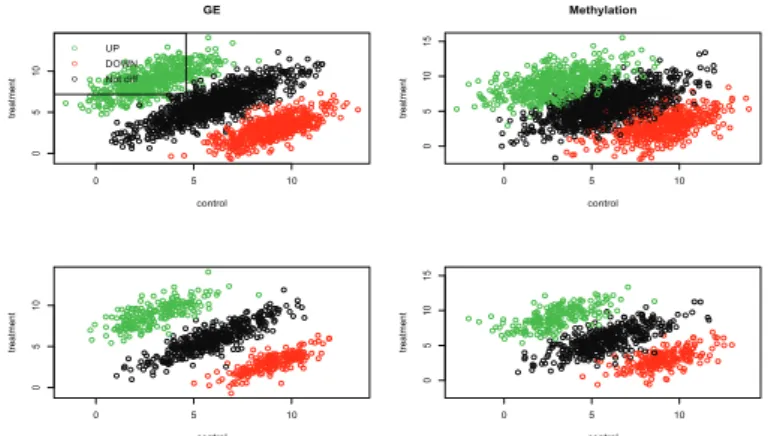
In this section, we evaluate our method through simulation study. We generate data that mimics the structure of real data as much as possible given in the next section. Structural similarity is summarized as follows: (1) data were generated based on normality assumption, (2) we consider two groups such as case and control, (3) within each group, gene expression has four replication, but no replicate for methylation, and (4) each gene has a couple of probes ranging from 1 to 4.

4.1. Simulation setup

The data are generated jointly by using pre-specified values given below.

• The number of genes: 800.

• Each gene has a few probes: 1 ∼ 4.

The true parameter values are given:

ρ = (1, 2, 1, 2, 4, 2, 1, 2, 1)/16, σ ² = 0.81, δ ² = 1.96, ω ² = 0.64, τ ² = 1.44,

Σ 1 =



 

 

1 0.9 0.1 0.1 0.9 1 0.1 0.1 0.1 0.1 1 0.9 0.1 0.1 0.9 1



 

  , µ 1 =



 

  9 3 9 3



 

  , Σ 2 =



 

 

1 0.9 0.1 0.1 0.9 1 0.1 0.1 0.1 0.1 2 1.8 0.1 0.1 1.8 2



 

  , µ 2 =



 

  9 3 6 6



 

  ,

Σ 3 =



 

 

1 0.9 0.1 0.1 0.9 1 0.1 0.1 0.1 0.1 1.5 1.2 0.1 0.1 1.2 1.5



 

  , µ 3 =



 

  9 3 3 9



 

  , Σ 4 =



 

 

2 1.8 0.1 0.1 1.8 2 0.1 0.1 0.1 0.1 1 0.9 0.1 0.1 0.9 1



 

  , µ 4 =



 

  6 6 9 3



 

  ,

Σ 5 =



 

 

2 1.8 0.1 0.1 1.8 2 0.1 0.1 0.1 0.1 2 1.8 0.1 0.1 1.8 2



 

  , µ 5 =



 

  6 6 6 6



 

  , Σ 6 =



 

 

2 1.8 0.1 0.1 1.8 2 0.1 0.1 0.1 0.1 1.5 1.2 0.1 0.1 1.2 1.5



 

  , µ 6 =



 

  6 6 3 9



 

  ,

0 5 10

0510

GE

control

treatment

o o o

UP DOWN Not diff

0 5 10

051015

Methylation

control

treatment

0 5 10

0510

control

treatment

0 5 10

051015

control

treatment

Figure 4.1. Simulated data; top: gene expression(left) and methylation(right) at the probe level; bottom: gene expression(left) and methylation(right) at the gene level

Table 4.1. Simulated data: Parameter estimates

Parameter True value Parameter estimates

(ρ 1 , ρ 2 , ρ 3 ) (0.0625, 0.125, 0.0625) (0.06625, 0.11750, 0.06750) (ρ 4 , ρ 5 , ρ 6 ) (0.1250, 0.250, 0.1250) (0.12750, 0.23625, 0.13375) (ρ 7 , ρ 8 , ρ 9 ) (0.0625, 0.125, 0.0625) (0.07000, 0.12125, 0.06000)

(δ ² , τ ² ) (1.96, 1.44) (1.9385, 1.3358)

(σ ² , ω ² ) (0.81, 0.64) (0.8395, 0.7208)

(µ 11 , µ 12 ) (9, 3) (9.3237, 3.2087)

(µ 41 , µ 42 ) (6, 6) (5.8922, 5.9481)

(µ 71 , µ 72 ) (3, 9) (3.0097, 9.0770)

(η 11 , η 12 ) (9, 3) (8.6763, 2.6672)

(η 21 , η 22 ) (6, 6) (5.6981, 5.5928)

(η 31 , η 32 ) (3, 9) (2.9341, 8.8845)

Σ 7 =



 

 

1.5 1.2 0.1 0.1 1.2 1.5 0.1 0.1 0.1 0.1 1 0.9 0.1 0.1 0.9 1



 

  , µ 7 =



 

  3 9 9 3



 

  , Σ 8 =



 

 

1.5 1.2 0.1 0.1 1.2 1.5 0.1 0.1 0.1 0.1 2 1.8 0.1 0.1 1.8 2



 

  , µ 8 =



 

  3 9 6 6



 

  ,

Σ 9 =



 

 

1.5 1.2 0.1 0.1 1.2 1.5 0.1 0.1 0.1 0.1 1.5 1.2 0.1 0.1 1.2 1.5



 

  , µ 9 =



 

  3 9 3 9



 

  .

The simulated data obtained by using the values above are given in Figure 4.1.

Here we consider the iteration size of 300. Parameter estimates are summarized in Table 4.1 in order to check the accuracy of our method

Since our estimates are very close to the true value of each parameter, we are sure that our method

is working very well under the condition that our assumption is correct. In addition, we checked the

accuracy of the assignment. To this end, we apply a cutoff value to the posterior probability that

each gene belongs to each category. Here we consider a stringent cutoff value of 0.9. Assignment

results are summarized in the Table 4.2. As we can see, our method correctly assigns 769 genes out

of 800, i.e., accuracy is more than 96%(796/800 = 0.96125).

Table 4.2. Simulated data: The results of category assignment; NG: number of genes(true value), NAG: number of assigned genes, NCA: number of correctly assigned genes, NIA: number of incorrectly assigned genes

Cutoff = 0.9 C1 C2 C3 C4 C5 C6 C7 C8 C9 Tot

NG 50 100 50 100 200 100 50 100 50 800

NAG 53 94 54 102 189 107 56 97 48 800

NCA 50 94 50 97 186 99 50 95 48 769

NIA 3 0 4 5 3 8 6 2 0 31

Table 5.1. GE data structure

Group 1 Group 2

k = 1 k = 2 k = 3 k = 4 k = 1 k = 2 k = 3 k = 4

Gene 1

b 11 G 1111 G 1121 G 1131 G 1141 G 1112 G 1122 G 1132 G 1142

b 12 G 1211 G 1221 G 1231 G 1241 G 1212 G 1222 G 1232 G 1242

. . .

. . .

. . .

. . .

. . .

. . .

. . .

. . .

. . . b 1J ₁ G 1J ₁ 11 G 1J ₁ 21 G 1J ₁ 31 G 1J ₁ 41 G 1J ₁ 12 G 1J ₁ 22 G 1J ₁ 32 G 1J ₁ 42

. . .

. . .

. . .

. . .

. . .

. . .

. . .

. . .

. . .

. . .

Gene I

b I1 G I111 G I121 G I131 G I141 G I112 G I122 G I132 G I142

b I2 G I211 G I221 G I231 G I241 G I212 G I222 G I232 G I242

. . .

. . .

. . .

. . .

. . .

. . .

. . .

. . .

. . . b IJ _I G IJ _I 11 G IJ _I 21 G IJ _I 31 G IJ _I 41 G IJ _I 12 G IJ _I 22 G IJ _I 32 G IJ _I 42

5. Application to Real Data

In the previous section, we noticed that our method is working well when our assumption is correct.

In this section, we apply our method to real data: wild type and OHT resistant MCF7 breast cancer cell lines.

5.1. Data description (OHT versus WT)

For gene expression analysis, the Human Genome U133A 2.0 Array was used; in addition, dif- ferential methylation hybridization(DMH) was done using Affymetrix oligonucleotide microarrays.

Microarray Analysis Suite(MAS) version 5.0 was used for preprocessing. Experimental details were described in (Fan et al., 2006).

We compare two groups, wild type and OHT resistant cell line. Each group in gene expression has four replicates while each group in methylation has no replicate. GE data structure is given in the Table 5.1. We, however, restrict our attention to genes with at least two “present call” for gene expression and our focus to DNA methylation in the promoter region. Then, we select common genes existing in both data sets. As a result, gene expression data have 11286 probes at the probe level and 4078 genes at the gene level while methylation data have 10223 probes and 4078 genes.

The raw data plot is given in Figure 5.1.

5.2. Results

As an initial value for long chain, we use parameter estimates obtained from pilot study with

iteration size of 300. Based on the result of the parameter estimates, we estimate that the iteration

size of 2000 is enough to make sure the convergence of EM algorithm. As an illustration, trace plot

of four variance estimates are given in Figure 5.2.

Figure 5.1. Raw data plot

Figure 5.2. Four variance estimates

All parameter estimates are summarized in Table 5.2. Here ρ 1 , . . . , ρ 9 are proportion estimates corresponding to each category, respectively. The majority of the genes (30%) belong to Category 5 (C5).

At the category level, global association is summarized in Table 5.3.

In Table 5.3, it is clear that association is category-specific. For example, let us focus on the first row of the Table 5.3, correlation between wild type gene expression and wild type methylation.

Each category has totally different correlation estimates ranging from −0.61 to 0.95, implying that correlation is category-specific.

To examine the association at the gene level, we selected one category (say, Category 3) and cal-

culated gene-specific association three different ways as done in the global case: (1) correlation

between WT GE and WT Methylation, (2) correlation between resistant GE and resistant Methy-

lation, (3) correlation between difference in the two groups of GE and that of Methylation. In

Figure 5.3, three different histograms that show the distribution of local (gene-specific) associations

Table 5.2. Real data: Parameter estimates

Parameter Parameter estimates

(ρ 1 , ρ 2 , ρ 3 ) (0.1135, 0.0780, 0.0329)

(ρ 4 , ρ 5 , ρ 6 ) (0.1089, 0.2990, 0.0933)

(ρ 7 , ρ 8 , ρ 9 ) (0.1275, 0.1017, 0.0453)

(δ ² , τ ² ) (0.3514, 0.1024)

(σ ² , ω ² ) (5.3047, 2.5286)

(µ 11 , µ 12 ) (9.9819, 9.6381)

(µ 41 , µ 42 ) (11.1259, 11.1306)

(µ 71 , µ 72 ) (8.6259, 9.0194)

(η 11 , η 12 ) (8.1152, 7.6924)

(η 21 , η 22 ) (10.0419, 9.8902)

(η 31 , η 32 ) (8.7607, 9.2403)

Table 5.3. Estimated global correlation for nine category

Corr C1 C2 C3 C4 C5 C6 C7 C8 C9

Corr(GE W , M W ) 0.176 0.130 −0.081 0.264 0.379 0.947 −0.299 −0.607 −0.210 Corr(GE R , M R ) 0.228 0.635 0.299 0.366 0.427 0.890 −0.292 −0.680 −0.209 Corr(GE d , M d ) 0.237 0.041 −0.636 −0.554 −0.516 0.918 −0.930 −0.720 −0.256

Figure 5.3. Histogram of local correlation for category 3: left(correlation between gene expression wild type and methylation wild type); center(correlation between gene expression resistant and methylation resistant); right(correlation between gene expression difference and methylation difference)

are given. As we can see, the local correlations from each gene are widely distributed, implying that correlation is gene-specific.

As an illustrating example, we selected gene CDH3 that is very crucial in breast cancer studies. It is well known that the CDH3 gene, which act as a tumor suppressor gene, is hypomethylated in breast cancer. Our method assigned the gene to Category 4 (no change in GE and hypomethylation). Es- timated mean of the gene is ˆ µ = (10.338, 10.417, 6.754, 5.113) where µ = (µ GE _W , µ GE _R , η M _W , η M _R ).

Furthermore, at the category level, Corr 4 (GE d , M d ) = −0.554 and local association for the gene

CDH3, Corr CDH3 (GE d , M d ) was −0.272. Even though there is weak signal, our results are consistent

with the general understanding that hypomethylated genes are more likely to be upregulated.

6. Conclusion

In this article, we constructed hierarchical Bayes model to get clear insight on the interplay between gene expression and DNA methylation in promoter region. Our model provides a global (category- specific) and local (gene-specific) view on association, and such rich information might be used for an understanding of epigenetic therapy, leading to the important part of drug discovery. For example, through the restoration of DNA methylation patterns, we may make cancer cells respond back to the treatment.

Our results show that category-specific (global) correlation varies from category to category (for example, Corr(GE W , M W ) ranges from −0.6 to 0.9 in Table 5.3). In addition, within each cate- gory (say, Category 3), the distributions of three different types of local correlations are different.

Collectively, our results show that association between gene expression and DNA methylation is category-specific and gene-specific as well.

Applying a cutoff value to the posterior probability of each gene, our method assigns each gene to one of nine categories. After such gene assignment, we may focus on subset of genes that are assigned to a category of interest, especially, hypomethylated categories (say, Category 1, 4, 7) for breast cancer studies. Then those genes can be used for further study such as gene set analysis and gene pathway analysis. Since tens of thousands of genes are overwhelming for such analysis, our method plays a key role of narrowing the number of genes to produce an appropriate number of genes for following studies.

Acknowledgements

I am grateful to the Changyu Shen for helpful comments as well as to Kenneth Nephew for the data.

References

Ahuja, N., Mohan, A. L., Li, Q., Stolker, J. M., Herman, J. G., Hamilton, S. R., Baylin, S. B. and Issa, J.

J. (1997). Association between CpG island methylation and microsatellite instability in colorectal cancer, Cancer Research, 57, 3370.

Baylin, S. B. and Herman, J. G. (2000). DNA hypermethylation in tumorigenesis: Epigenetics joins genetics, Trends Genetics, 16, 168–174.

Bird, A. (2002). DNA methylation patterns and epigenetic memory, Gene Development, 16, 6–21.

Day, N. E. (1969). Estimating the components of a mixture of two normal distributions, Biometrika, 56, 463–474.

Dempster, A. P., Laird, N. M. and Rubin, D. B. (1977). Maximum likelihood from incomplete data via the EM algorithm, Journal of Royal Statistical Society B, 39, 1–38.

Dwivedi, R. S., Qiu, Y. Y., Devine, J. and Mirkin, B. L. (2003). Role of DNA methylation in acquired drug resistance in neuroblastoma tumors, Proceedings of Indian National Science Academy, 69, 111–120.

Esteller, M., Hamilton, S. R., Burger, P. C., Baylin, S. B. and Herman, J. B. (1999). Inactivation of the DNA repair gene O6-Methylguanine-DNA methyltransferase by promoter hypermethylation is a common event in primary human neoplasia, Cancer Research, 59, 793.

Fan, M., Yan, P. S., Hartman, F. C., Chen, L., Paik, H., Oyer, S. L., Salisbury, J. D., Cheng, A. S., Li, L., Abbosh, P. H., Huang, T. H. and Nephew, K. P. (2006). Diverse gene expression and DNA methylation pro thisfiles correlate with differential adaptation of breast cancer cells to the antiestrogens Tamoxifen and Fulvestrant, Cancer Research, 66, 11954–11966.

Figueiredo, A. T. M. and Jain, A. K. (2002). Unsupervised learning of finite mixture models, IEEE Trans-

actions on Pattern Analysis and Machine Intelligence, 24, 381–396.

George, C. (1985). An introduction to empirical bayes data analysis, American Statistician, 39, 83–87.

Herman, J. G. (1999). Hypermethylation of tumor suppressor genes in cancer, Seminars of Cancer Biology, 9, 359–367.

Herman, J. G. and Baylin, S. B. (2003). Gene silencing in cancer in association with promoter hypermethy- lation, New England Journal of Medicine, 349, 2042–2054.

Hinshelwood, R. A. and Clark, S. J. (2008). Breast cancer epigenetics: normal human mammary epithelial cells as a model system, Journal of Molecular Medicine, 86, 1315–1328.

Hui, R., Macmillan, R. D., Kenny, F. S., Musgrove, E. A., Blamey, R. W., Nicholson, R. I., Robertson, J.

F. and Sutherland, R. L. (2000). INK4a gene expression and methylation in primary breast cancer:

Overexpression of p16INK4a messenger RNA is a marker of poor prognosis, Clinical Cancer Research, 6, 2777.

Jeong, J., Li, L., Liu, Y., Nephew, K. P., Huang, T. H. and Shen, C. (2010). An empirical Bayes model for gene expression and methylation profiles in antiestrogen resistant breast cancer, BMC Medical Genomics, 3, 55.

Jones, P. A. and Baylin, S. B. (2007). The epigenomics of cancer, Cell, 128, 683–692.

Jones, P. A. and Laird, P. W. (1999). Cancer-epigenetics comes of age, Nature Genetics, 21, 163–167.

McLachlan, G. J. and Krishnan, T. (2007). The EM Algorithm and Extensions, John Wiley & Sons, New Jersey.

Muller, S., Fong, K. M., Maitra, A., Lam, S., Geradts, J., Ashfaq, R., Virmani, A. K., Milchgrub, S., Gazdar, A. F. and Minna, J. D. (2001). 5’ CpG island methylation of the FHIT gene is correlated with loss of gene expression in lung and breast cancer, Caner Research, 61, 3581.

Sundberg, R. (1974). Maximum likelihood theory for incomplete data from an exponential family, Scandi- navian Journal of Statistics, 1, 49–58.

Sundberg, R. (1976). An iterative method for solution of the likelihood equations for incomplete data from exponential families, Communications in Statistics-Simulation and Computation, 5, 55-64.

Wang, X., Chao, L., Jin, G., Ma, G., Zang, Y. and Sun, J. (2009). Association between CpG island methylation of the WWOX gene and its expression in breast cancers, Tumor Biology, 30, 8–14.

Wu, C. F. J. (1983). On the convergence properties of the EM algorithm, Annals of Statistics, 11, 95–103.

Xu, L. and Jordan, M. I. (1996). On convergence properties of the EM algorithm for Gaussian mixtures,

Neural Computation, 8, 129–151.