*준회원, 울산대학교 전기전자컴퓨터공학과
**정회원, 울산대학교 IT융합학부(교신저자)
접수일자: 2018년 3월 18일, 수정완료: 2018년 4월 5일 게재확정일자: 2018년 4월 6일
Received: 18 March, 2018 / Revised: 5 April, 2018 Accepted: 6 April, 2018
**Corresponding Author: [email protected] School of IT Convergence, University of Ulsan, Korea https://doi.org/10.7236/JIIBC.2018.18.2.169
JIIBC 2018-2-21
무선네트워크에서의 지연시간제약을 고려한 듀티사이클 스케쥴링
Duty Cycle Scheduling considering Delay Time Constraints in Wireless Sensor Networks
부쥐손*, 윤석훈**
Vu Duy Son*, Seokhoon Yoon**
요 약 본 논문에서는 센서노드가 전력소모를 줄이기 위하여 주기적으로 휴면상태를 갖는 듀티사이클 기반 무선센서 네트워크를 고려한다. 이러한 네트워크에서는 듀티사이클 간격이 커진다면 전력소모는 감소하지만 종단간 지연시간은 늘어나게 된다. 무선센서네트워크의 많은 애플리케이션은 지연시간에 민감하며 패킷이 센서노드로부터 싱크노드에게 전 달되는 데 있어서 지연시간제약 요구사항이 있다. 기존의 대부분의 연구는 종단간 지연시간을 줄이는 것에만 초점을 맞추고 지연시간제약에 대해 고려를 하지 않음으로써 종단간지연시간과 전력소모에 대한 균형을 맞추기 어려웠다. 지연 시간제약을 고려하는 연구에서도 노드들간의 시각동기화를 요구하거나 노드들이 특정한 분포를 갖는다고 가정하였다.
기존 연구의 이러한 제약을 극복하기 위하여 본 논문에서는 지연시간제약조건을 충족시키면서 동시에 전력소모를 줄이 기 위한 듀티사이클 스케쥴링 알고리즘을 제안한다. 먼저 종단간 지연시간의 확률분포를 추정하고 획득한 분포를 이용 하여 지연시간제약조건을 만족하는 최대 듀티사이클 간격을 결정한다. 시뮬레이션 결과에 따르면 제안되는 알고리즘은 주어진 지연시간제약 요구사항을 만족하면서도 낮은 전력소모 성능을 보인다.
Abstract In this paper, we consider duty-cycled wireless sensor networks (WSNs) in which sensor nodes are periodically dormant in order to reduce energy consumption. In such networks, as the duty cycle interval increases, the energy consumption decreases. However, a higher duty cycle interval leads to the increase in the end-to-end (E2E) delay. Many applications of WSNs are delay-sensitive and require packets to be delivered from the sensr nodes to the sink with delay requirements. Most of existing studies focus on only reducing the E2E delay, rather than considering the delay bound requirement, which makes hard to achieve the balanced performance between E2E delay and energy consumption. A few study that considered delay bound requirement require time synchronization between neighboring nodes or a specific distribution of deployed nodes. In order to address limitations of existing works, we propose a duty-cycle scheduling algorithm that aims to achieve low energy consumption, while satisfying the delay requirements. To that end, we first estimate the probability distribution for the E2E delay. Then, by using the obtained distribution we determine the maximal duty cycle interval that still satisfies the delay constraint.
Simulation results show that the proposed design can satisfy the given delay bound requirements while achieving low energy consumption.
Key words : Wireless sensor networks, Duty cycling, Delay bound, Deadline success ratio.
I. Introduction
Recently, wireless sensor networks (WSNs) have been widely used for many applications such as health monitoring, target tracking, and environmental monitoring[1-2]. In WSNs, sensors are deployed in a region to sense and measure environmental parameters such as concentration of toxic materials, gas, and temperature. Since the primary power source of a sensor node is a battery with limited capacity, saving power consumption is essential in WSNs. One of the most effective techniques for reducing energy consumption in WSNs is the duty cycling mechanism
[3-6]
.
Unfortunately, the increase in the duty cycle interval for saving energy leads to a long E2E delay[7]. Most delay-sensitive applications require that packets reach the sink within a given delay bound. However, most of existing studies only considered minimizing the E2E delay[8-10], rather than taking the delay bound and energy consumption into consideration at the same time.
Although a few studies considered both the delay bound and energy consumption, they require additional information or certain assumptions. For example, Z.
Fan et al. [10] proposed a transmission power control mechanism to satisfy the given delay bound. However, nodes need to know wake-up schedules of all neighboring nodes. Dao et al. [11] also considered those requirements, but this scheme is only applied to random deployment of WSN nodes in a circular area and not applicable to various practical deployments.
In order to address limitations of existing studies, we propose a delay-constrained duty-cycle scheduling algorithm (DDS) that aims to achieve low energy consumption, while satisfying the delay requirements.
The main idea of our work is that maximizing the duty cycle interval with the constraint of the delay bound.
We define deadline success ratio (DSR) as the required probability which is the ratio between the number of packets delivered to the sink within a given
delay bound and the total number of transmitted packets. For example, an application needs 95 % (the required DSR) of the transmitted packets to arrive at the sink within 30 seconds (the delay bound). Firstly, the E2E delay distribution is estimated as a function of the duty cycle interval. Then, we propose four methods to obtain maximal duty cycle interval values that satisfies the required DSR. In addition, our algorithm does not require time synchronization between neighboring nodes and can be applied to various deployment strategies in WSNs, e.g., circular or rectangular areas, random or manual deployment. The simulation results show that the network performance can satisfy both the given delay bound and required DSR.
The rest of the paper is design as follows: Section II introduces the network model and defines an optimization problem. Our proposed scheme is presented in Section III. The evaluation of simulation results are shown in Section IV, and the paper is concluded in Section V.
II. Network Model and Problem Definition
Firstly, this section introduces the system model for duty-cycled WSNs, then a maximization problem for estimating the maximal duty cycle interval that satisfies delay requirements is presented.
We consider a WSN that uses multi-hop transmission and includes static sensor nodes including a sink node with transmission range . Our design can be applied to various deployment strategies, for example, the sensor’s deployment area can be circular or rectangular regions, random or manual deployment. Because of the duty cycling mechanism, nodes are active or dormant during a duty cycle interval except for the sink which is always active. In addition, when a node detects an event, the node will turn on the radio to transmit packets if it is in the sleep
state. Let and denote the duty cycle interval and the active period of nodes in , respectively. For a duty cycle interval, sensor nodes randomly and independently select the time to wake up. Hence, the wake-up schedules of nodes are asynchronous. In other words, time synchronization is not required for our work.
For duty-cycled WSNs, the one-hop delay of a node depends on the wake/sleep schedules of forwarding candidates, hence it is influenced by the duty cycle interval. Furthermore, the one-hop delay also depends on other network parameters, e.g., the transmission range of nodes, the number of neighboring nodes, and the number of forwarders. Because the E2E delay is the sum of one-hop delay, the E2E delay depends on the duty cycle interval and network parameters. Let and denote the given delay bound of packets’ E2E delay and the required DSR, respectively. We define a delay duty-cycling maximization problem as follows.
The objective of this problem is the maximization of the duty cycle interval , and the constraint is that the ratio between packets arrived at the sink within the given delay bound and the total transmitted packets is greater than or equal the required DSR .
III. Delay-constrained Duty-cycle Scheduling Algorithm
In this section, we propose a novel scheduling algorithm that maximizes the duty cycle interval while guaranteeing the given delay bound with the required DSR. Firstly, we estimate the E2E delay distribution, then the duty cycle interval is determined based on the estimated E2E delay distribution.
1. Estimation of End to End Delay Distribution
In this subsection, we first estimate the one-hop delay distribution in each group because the E2E delay is the sum of one-hop delay. Then we propose methods
for estimating the E2E delay distribution that is formulated as a function of the duty cycle interval and network parameters.
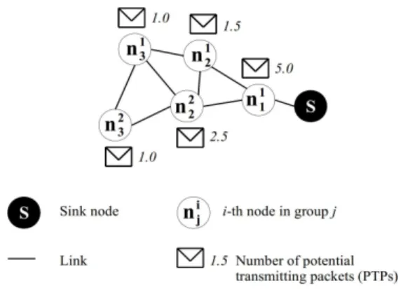
그림 1. 잠재적 전송 패킷 예시
Fig. 1. An example of potential transmitting packets.
We introduce important definitions as follows. Let
and define -th node and the number of nodes in group , respectively. Let potential forwarding candidate(s) (PFCs) of node define nodes that relay packets of node to the sink. In order to facilitate the discussion, suppose that every node generates only one packet, and all packets are successfully delivered to the sink. A node not only transmits its packets but also forwards packets received from other nodes. Let potential transmitting packet(s) (PTPs) define packets that a node needs to forward to the sink. Let and
denote the number of PFCs and PTPs, respectively.
The number of PTPs depends on the number of PFCs.
For example, as can be seen in Fig. 1, because node does not forward packets of other nodes.
Meanwhile, node needs to forward its packets and node ’s packets. In addition, node has two PFCs and one PTP, hence probably transmits 0.5 packets to , hence PTPs.
Suppose that the group index of all nodes is determined and the sink is aware of nodes’ information that will be used to estimate the E2E delay distribution,
e.g., group index, the number of PFCs, and the number of PTPs.
The larger number of PTPs of a node, the higher probability that this node is selected to relay packets can be achieved. Let denote the number of PTPs of nodes in group . Hence, the probability that is selected can be calculated as follows:
(1)
Let define a one-hop delay random variable which is the latency of packets from hop to previous hop
. Note that where is the maximum hop count, and the hop count of the sink is zero. Let
denote the probability that the one-hop delay of node is shorter than when selecting to forward packets. Nodes randomly and independently wake up during a duty cycle interval. A transmitter chooses the first wake-up node among PFCs to forward packets. In addition, the sink is aware of node’s information, e.g., the number of PFCs of nodes.
Hence, we obtain:
(2)
One-hop delay distribution not only depends on the wake-up time of PFCs but also depends on the number of PTPs. If packets are transmitted by a node that has a longer one-hop delay, it is more probable that the E2E delay of these packets is larger. Therefore, we estimate the cumulative distribution function of one-hop delay using Bayes’ theorem as follows:
(3)
According to Eq. (3), probability density function is expressed as follows:
(4)
The mean and variance of the one-hop delay are calculated as follows:
(5)
(6)
where
(7)
(8)
Let be a random variable which denotes the E2E delay of packets which is the sum of one-hop delay.
Furthermore, we consider the E2E delay in the worst case in which the E2E delay is calculated for packets whose hop count is the maximum. Note that the sink is always active, in other words, . Therefore, the E2E delay is expressed as follows:
(9)
We approximate the E2E delay distribution by the sum of one-hop delay distribution :
′ (10)
where is a distribution that represents all one-hop delay distribution of groups. If ′ satisfies the given delay bound, also satisfies. In order to find the
representative of one-hop delay distribution of groups, we propose four methods that based on the selection of
from obtained one-hop delay distribution and estimation of as a new distribution.
1.1 Selection of from obtained one-hop delay distribution
We propose two methods for choosing a representative one-hop delay distribution from obtained one-hop delay distribution as follows:
(i) Mean: The mean value of a one-hop delay distribution represents the central tendency of the one-hop delay value. A group has a higher mean value, it is more probable that this group has a longer delay time. We select the group with the largest mean value.
(ii) The product of mean and standard deviation (PMS): With the probabilistic approach, the E2E delay values in practice are spread out over a long range. Some delay values can be very large compared to the mean value. Therefore, we take standard deviation into consideration. If the standard deviation of E2E delay distribution of a group is more significant, the maximum value of E2E delay can be larger. We define the product of mean and standard deviation . We select the group that has the largest value of PMS.
1.2 Estimation of as a new distribution Instead of selecting one-hop delay distribution from obtained distribution, we estimate a new distribution which is a mixture of all one-hop delay distribution using a finite mixture model[12]. From our experiments, with randomly generated position of sensors, it seems that the probability density function of the one-hop delay distribution of each group follows an exponential distribution with the mean value
of the distribution of group is derived from information at the sink according to Eq. (7). The finite
mixture model for components is expressed as follows:
(11)
where is the mixing proportion or weight;
≤ ≤ , and
.
To determine values of the mixing weights, we propose two methods which are estimation of with same weights and different weights.
(i) Estimation of with same weights (ESW): All weights have value .
(ii) Estimation of with different weights (EDW):
The weight values of distribution are not the same and depend on the number of PTPs of all nodes in the same group:
(12)
where is the number of PTPs of nodes in group .
2. Determination of duty cycle interval using estimated E2E delay distribution After estimating the one-hop delay distribution, we approximate the E2E delay using the classic central limit theorem. The mean and variance
of one-hop delay are calculated by Eq. (7) and Eq. (8), respectively. The maximal duty cycle interval
that satisfies the given delay bound and required DSR is expressed as follows:
(13)
where stands for the required DSR.
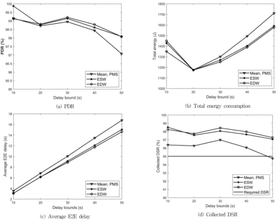
(a) PDR (b) Total energy consumption
(c) Average E2E delay (d) Collected DSR
그림 2. 지연 제약 변화의 PDR, 총전력소모, 평균종단지연 및 수집된 DSR에의 영향
Fig. 2. Impact of delay bound on PDR, total energy consumption, average E2E delay, and collected DSR.
IV. Performance Results
In this section, the simulation setup and the performance results of DDS are presented. We simulate a network using the ns-2 simulator [13]. To evaluate four methods (mean, PMS, ESW, and EDW), we consider the evaluation metrics under the impact of delay bounds.
1. Simulation Setup
In this section, the network parameters were set as follows. Seventy-eight nodes are deployed in the rectangular region (40 m x 50 m) with the sink is in the center region. The transmission range is 10 m and the maximum group index is 6. Assume that Preon32 [14]
- the radio module of the sensor nodes is used with high bandwidth (2 Mbps). For this node deployment
and position of the sink, the selection of based on the mean and PMS methods are the same, hence the results of both are identical. We simulate with the scenario in which a randomly selected node transmits a 46 bytes data packet every 1 s (event rate = 1.0 packet/s).
To validate the proposed methods, we analyze the network performance under following evaluation metrics: average E2E delay, total energy consumption of all nodes, PDR, and collected DSR. We study the effect of the delay bound on different evaluation metrics. The delay bounds are [10 20 30 40 50] s with the required DSR .
2. Evaluation Results
The network performance with varied delay bounds is illustrated in Fig. 2. As can be seen in Fig. 2(a), PDR
is higher than 97% over different delay bounds. PDR slightly decreases when the delay bound increases. The reason is as follows. When the duty cycle is higher, the waiting time increases. If the waiting time is longer, there is a higher probability that the nodes are busy when other nodes try to transmit packets. If the packet is dropped because of exceeding the number of retransmissions, PDR decreases. In addition, the PDR of EDW achieves the highest value when the delay bound is greater than 20 s.
As can be seen in Fig. 2(b), the energy consumption of all methods achieved the minimal value with the delay bound s and the pattern follows a V-shape. The reason is as follows. When the delay bound is varied from 10 s to 20 s, the duty cycle interval increases because the duty cycle interval is directly proportional to the delay bound according to Eq. (13). For the same active period, the higher duty cycle interval, the smaller energy consumption can be achieved. In contrast, when the delay bound is changed from 20 s to 50 s, the energy consumption increases.
While the active period and event rate are not changed, increasing in the duty cycle interval leads to the collision because several transmitters try to send many packets to one node. These transmitters need to be active for a longer period to retransmit packets, hence the energy consumption increases. In addition, the total energy consumption of EDW achieves the lowest value with the delay bound is varied from 30 s to 50 s.
In terms of average E2E delay, as shown in Fig.
2(c), all methods satisfy the given delay bound. The average E2E delay increases when the delay bound increases. The reason is as follows. The delay bound is directly proportional to the duty cycle interval.
Furthermore, the longer average E2E delay, the higher duty cycle interval can be achieved. Fig. 2(d) shows the collected DSR results with varied delay bound values. Mean and PMS methods do not satisfy the required DSR with the given delay bound
s. Meanwhile, other proposed methods satisfy the required DSR. Note that EDW can achieve the
collected DSR with the highest value.
In summary, the network performance of EDW is better than that of the other methods. The average E2E delay of four proposed methods satisfies the given delay bound. In terms of collected DSR, both ESW and EDW methods always satisfy the required DSR. The collected DSR of the mean and PMS methods satisfy the required DSR with the delay bounds varied from 10s to 40 s and does not satisfy the one with delay bound s.
V. Conclusion
In this paper, we proposed a novel scheduling algorithm to estimate the maximal duty cycle intervals that satisfy the delay requirements such as a given delay bound and required deadline success ratio for duty-cycled WSNs. To do that, we estimate the E2E delay distribution as a function of the duty cycle interval and network parameters. Furthermore, our design can be applied to different deployment strategies of WSNs, hence the calculated duty cycle interval is more adaptive for practical applications. The simulation results demonstrate that our values of the duty cycle interval can satisfy the delay requirements.
References
[1] P. Rawat, K. D. Singh, H. Chaouchi, and J. Bonnin,
“Wireless sensor networks: a survey on recent developments and potential synergies,” The Journal of Supercomputing, vol. 68, no. 1, pp.
1-48, Apr 2014.
[2] W. Y. Chang, Y. C. Lee, and J. J. Kang,
“Implementation of IoT sensors network using mobius platform,” The Journal of The Institute of Internet, Broadcasting and Communication (JIIBC), vol. 17, no. 2, pp. 211-218, April 2017.
[3] J. Hao, B. Zhang, and H. T. Mouftah, “Routing protocols for duty cycled wireless sensor networks:
※ 이 논문은 2016년도 정부(교육부)의 재원으로 한국연구재단의 지원을 받아 수행된 기초연구사업임(No.
2016R1D1A3B03934617)
A survey,” IEEE Communications Magazine, vol.
50, no. 12, pp. 116-123, December 2012.
[4] Y. Gu and T. He, “Dynamic switching-based data forwarding for low-duty-cycle wireless sensor networks,” IEEE Transactions on Mobile Computing, vol. 10, no. 12, pp. 1741-1754, Dec 2011.
[5] C. J. Merlin and W. B. Heinzelman, “Node synchronization for minimizing delay and energy consumption in low-power listening mac protocols,” in 2008 5th IEEE International Conference on Mobile Ad Hoc and Sensor Systems, Sept 2008, pp. 265-274.
[6] J. Jung, J. Yoon, Y. Yun, S. So, and S. Eun, “A dynamic duty cycle adjustment mechanism for reduced latency in industrial plants,” The Journal of The Institute of Internet, Broadcasting and Communication (JIIBC), vol. 16, no. 1, pp.
193-198, February 2016.
[7] R. C. Carrano, D. Passos, L. C. S. Magalhaes, and C. V. N. Albuquerque, “Survey and taxonomy of duty cycling mechanisms in wireless sensor networks,” IEEE Communications Surveys Tutorials, vol. 16, no. 1, pp. 181-194, First 2014.
[8] J. Kim, X. Lin, N. B. Shroff, and P. Sinha,
“Minimizing delay and maximizing lifetime for wireless sensor networks with anycast,”
IEEE/ACM Transactions on Networking, vol. 18, no. 2, pp. 515-528, April 2010.
[9] B. Nazir and H. Hasbullah, “Dynamic sleep scheduling for minimizing delay in wireless sensor network,” in 2011 Saudi International Electronics, Communications and Photonics Conference (SIECPC), April 2011, pp. 1-5.
[10] Z. Fan, S. Bai, S. Wang, and T. He,
“Delay-bounded transmission power control for low-duty-cycle sensor networks,” IEEE Transactions on Wireless Communications, vol.
14, no. 6, pp. 3157-3170, June 2015.
[11] T. N. Dao, S. Yoon, and J. Kim, “A deadline-aware scheduling and forwarding scheme in wireless sensor networks,” Sensors, vol. 16, no. 1, 2016.
[12] G. McLachlan, “Finite mixture models [electronic resource],” Hoboken, 2004.
[13] “Network simulator,” accessed 03-2018. Available:
https://www.isi.edu/nsnam/ns/
[14] Virtenio, “Preon32 wireless module datasheet,”
accessed 03-2018.
Available: https://www.virtenio.com
저자 소개
부 쥐 손(준회원)
∙August, 2015 : B. Sc in Electronics and Telecommunications Engineering, School of Electronics and Telecommunications, Hanoi University of Science and Technology, Vietnam
∙Sep. 2016 ∼ Present : MS Student in Dept. of Electrical and Computer Engineering, University of Ulsan
<Research Interests : Wireless Sensor Network, Ad hoc Network>
윤 석 훈(정회원)
∙February, 2000 : B.E in automation engineering, Inha University
∙June, 2005 : M.S in Computer Science and Engineering, SUNY at Buffalo
∙September, 2009 : Ph.D. in Computer Science and Engineering, SUNY at Buffalo
∙2009 ∼ 2011 : Senior Researcher, LIG Nexone
∙2011 ∼ present : Associate Professor, University of Ulsan <Research Interests : Intelligence defined networking, Machine learning based IoT systems, Wireless Sensor Networks>