* Corresponding author: (E-mail) [email protected]
※Advance in Forest Management and Inventory-selected papers from the international conference of IUFRO (Div. 4.01, 4.02, 4.04), Chuncheon, Korea, Oct. 13-17, 2008.
Economic Analysis of Snow Damage on Sugi
( Cryptomeria japonica ) Forest Stands in Japan Within the Forest Stand Optimization Framework
Atsushi Yoshimoto1, Akio Kato2, and Hirokazu Yanagihara3*
1Dept. of Math. Analy. and Stats. Infer., Institute of Statistical Mathematics, Tokyo, Japan, [email protected]
2Toyama Prefectural Agricultural, Forestry & Fisheries Research Center, Toyama, Japan, [email protected]
3Dept. of Mathematics, Hiroshima University, Hiroshima, Japan, [email protected]
ABSTRACT : We conduct economic analysis of the snow damage on sugi (Cryptomeria japonica) forest stands in Toyama Pre- fecture, Japan. We utilize a single tree and distant independent growth simulator called “Silv-Forest.” With this growth simulator, we developed an optimization model by dynamic programming, called DP-Silv (Dynamic Programming Silv-Forest). The MS- PATH (multiple stage projection alternative technique) algorithm was embedded as a searching algorithm of dynamic programming.
The height / DBH ratio was used to constrain the thinning regime for snow damage protection. The optimal rotation age turned out to be 65 years for the non-restricted case, while it was 50 years for the restricted case. The difference in NPV of these two cases as the induced costs ranged from 179,867 to 1,910,713yen/ha over the rotation age of 20 to 75 years. Under the optimal rotation of 65 years, the cost became 914,226 yen/ha. The estimated annual payment based on the difference in NPV, was from 9,869 yen/ha/yr to 85,900 yen/ha/yr. All in all, 10,000 yen/ha/yr to 20,000 yen/ha/yr seems to cover the payment from the rotation age of 35 to 75 years.
Keywords : Snow damage, Cryptomeria japonica, Algorithm, Forest management
INTRODUCTION
Snow damage on artificial forest stands has been one of the main concerns in snow regions, Japan. It breaks stems and branches with the large economic loss to forest owners. Kato et al. (1992) conducted the analysis on the ratio of height to DBH (diameter at breast height) (hereafter called H/D ratio) for a sugi (Cryptomeria japonica) forest stand against snow damage, and found out that the H/D ratio should be maintained less than 65% to avoid the damage under the thinning regime. Although this require- ment seems to reduce the benefits from the management, it could be offset by the benefits of avoiding the damage beforehand.
In this research, we conduct economic analysis of the
snow damage on sugi forest stands in Toyama Prefecture, Japan. We utilize a single tree and distant independent growth simulator called “Silv-Forest.” This growth simulator was originally developed by Tanaka (1995) and modified by Kato and Tanaka (1997) and Kato et al. (2008) for sugi forests in Toyama. One of the main characteristics of Silv-Forest is that the DBH distribution is first created from the observed data, then the distribution progresses mainly based on diameter growth at each DBH class following the normal distribution with the derived mean of growth and the given coefficient of variation for growth.
It has been used on the spreadsheet basis of Microsoft Excel Software. With some arrangements, we modify it further to be optimized for the thinning regime after converting it into the FORTRAN programming language.
With this growth simulator, we develop an optimization model by dynamic programming, called DP-Silv (Dynamic Programming Silv-Forest). The MS-PATH (multiple stage projection alternative technique) algorithm is embedded as a searching algorithm of dynamic programming. The H/D ratio is used to constrain the thinning regime for snow damage protection. The paper is organized as follows. In the second section, the MS-PATH algorithm is mathemati- cally elaborated. In the third section, we conduct econo- mic analysis on the snow damage, then some concluding remarks are provided in the last section.
Dynamic Programming Specification
The dynamic programming approach has been developed and extensively applied for optimizing thinning regimes (Arimizu, 1958a, b; Amidon and Akin, 1968; Schreuder, 1971; Kilkki and Väisänen, 1970; Adams and Ek, 1974;
Brodie et al., 1978; Brodie and Kao, 1979; Chen et al., 1980; Martin and Ek, 1981; Riitters et al., 1982; Brodie and Haight, 1985; Haight et al., 1985; Valsta and Brodie, 1985; Arthand and Klemperer, 1988; Torres and Brodie, 1990). However, as forest stand growth models were developed with growth complexity, the dynamic program- ming approach became inefficient for optimization due to vast increase in dimensionality for the state description of iteration called the curse of dimensionality.
While the curse of dimensionality had been the main problem for these early applications of dynamic pro- gramming. Paredes and Brodie (1987) introduced a new searching algorithm called PATH (Projection Alternative Technique) within the framework of both network theory and the theory of the Lagrange multipliers to resolve the problem. Their derivation of the algorithm was somewhat ad-hoc with difficulty of searching for optimal values of Lagrange multipliers. With the concept of calculus of variation, Yoshimoto et al. (1988) introduced a new deri- vation of the algorithm, and pointed out the shortcoming of PATH in considering a long-term effect of thinning activities on the objective function. They developed the
MS-PATH (Multiple Stage PATH) algorithm to overcome the problem by considering all possible future path com- bination. The recent application of MS-PATH can be found in Yoshimoto and Marušák (2007). In what follows, we elaborate the algorithm.
Let x(t) be a state variable representing a forest stand at time t, and ẋ(t) be its first derivative with respect to time t. Introducing a marginal function, π(․), of the objec- tive for the management, say, the net present value of the profits, over time, the objective is to maximize its integral from the initial state (plantation), x0 at time t0, to the end- ing state (final harvest) xn at time tn with respect to a control variable, ẋ(t).
{ ( )} 0
0 0
max ( ( ), ( ), ) ( )
( )
tn
x t t
n n
J x t x t t dt x t x
x t x π
=
=
=
&
∫
&(1) In the thinning management problem, thinning inten- sity, T(t) at time t is of the major concern, and controls x(t) and ẋ(t), so that the control variable can be replaced by thinning, T(t),
{ ( )} 0
0 0
max ( ( ), ( )) ( )
( )
tn
T t t
n n
J x t T t dt x t x
x t x π
=
=
=
∫
(2) Converting the objective function into the discrete thinning problem with thinning at age of t (t = t0, t1, …, tn), we have,
1 1
{ ( )} 1
0 0
max ( ( ) | ( ))
( ) ( )
i i i
n t
t i
T t i
n n
J x t T t dt
x t x x t x π
− −
=
=
=
=
∑∫
(3) Introducing the integrand of Π(x(ti)T(ti-1)) =
π(x(τ)T(ti-1))dτ, the objective function of equation becomes,
1
1
{ ( )} 1 1
1 0 1
1
max ( ( ) | ( ))
{ ( ( ) | ( )) ( ( ) | ( )) }
i i i
i
n t
t i
T t i
n t
i i i
i
J x t T t dt
x t T t x t T t dt π
π
−
−
−
=
− −
=
=
= Π −
∑∫
∑ ∫
(4)Let us introduce the contribution value function, ΠT(T(ti)), of thinning, T(ti), which satisfies the following,
0tiπ( ( ) | ( ))x t T t dti = Π( ( ) | (x ti T ti−1))− ΠT( ( ))T ti
∫
(5)The first term of the right-hand side is the contribution value of a forest stand, Π(․), at time ti after having thinn- ing T(ti-1) at time ti-1 and the second term is the amount taken by thinning T(ti) at time ti. As a result, the dif- ference is the contribution value of a stand just after hav- ing thinning at time ti. With equation (5), equation (4) becomes.
1
1 0 1
{ ( )} 1
1 1 1 2
1
max { ( ( ) | ( )) ( ( ) | ( )) }
{ ( ( ) | ( )) ( ( )) ( ( ) | ( ))}
i i
n t
i i i
T t i
n
T
i i i i i
i
J x t T t x t T t dt
x t T t T t x t T t
π
−
− −
=
− − − −
=
= Π −
= Π + Π − Π
∑ ∫
∑
(6) Note that only the first two terms on the right-hand side have affects from thinning, T(ti).
With one stage look-ahead search in the PATH algorithm (Paredes & Brodie, 1987), the following optimality equation is obtained.
1
*
{ } 1
* *
1 1 1 1 1
max{ ( )}
( ) ( ) ( )
i
i T i i
T
i i i i i i i
f f T
f T T T f
− −
− − − − −
=
= Π + Π − Π + (7)
where Ti= T(ti), Πi(Ti-1) = Π(x(ti)T(ti-1)), ΠT(Ti) = ΠT(T(ti)), Πi*= Πi(T*i-1), and Ti* is an optimal thinning intensity at time ti. Considering influence of thinning over multiple periods by MS-PATH, the optimality equation of MS- PATH becomes,
,
*
, ,
{ , }
* *
, , ,
max { ( )}
( ) ( ) ( )
i i j
i T j i i j i i j
i T
i j i i j i i i j i i j i j i j
f f T
f T T T f
− − −
− − − − − −
=
= Π + Π − Π + (8)
This is to search for an optimal thinning intensity as well as an optimal elapse of the stage, j, from the (i-j)-th
stage for two sequential thinning over multiple stages.
Note that Ti,i-j is thinning intensity at time ti-j with the elapse of the stage j from the i-th stage, Πi(Ti,i-j) is the contribution value of a forest stand at time ti after having thinning Ti,i-j at time ti-j, ΠT(Ti,i-j) is the contribution value of thinning Ti,i-j implemented at time ti-j, j* is an optimal elapse of the stage from the i-th stage, T*i,i-j is an optimal thinning intensity at time ti-j targeting time ti, Π*i= Π
(T*i,i-j*), is the contribution value of a forest stand at time
ti after having an optimal thinning intensity T*i,i-j* at time ti-j* with an optimal elapse of the stage j*. The algorithm searches for an optimal solution by maximizing the sum of the contribution value of a forest stand and thinning.
Analysis
Regarding the growth simulator of Silv-Forest, we im- plemented the following modification. First we utilized the relative taper curve function to estimate volume of a tree by every 1/10 segmentation of a tree. Second, since the original Silv-Forest did not consider self-thinning, we em- bedded it to the model.
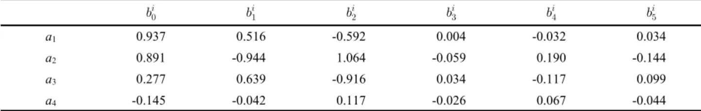
The taper curve function is to estimate the i-10 th rela- tive diameter size, Di to DBH, by the following empirical polynomial function of a relative height, xi, with all para- meters estimated as a function of the corresponding DBH and height, so that at each DBH class one unique taper curve is derived.
2 3 20
1 2 3 4 1,...,10
i i i i i
D = ⋅ + ⋅ + ⋅ + ⋅a x a x a x a x i= (9) Each parameter is a function of DBH and height defined by the following bilinear form.
2
0 1 2 3 4
i i i i i
i j j j j j
a = + ⋅b b H + ⋅b DBH + ⋅b H + ⋅b H DBH⋅ + 5 2
i
b DBHj
+ ⋅ (10)
Converting these equations into the framework of the estimated generalized least square (EGLS) estimation (see Vonesh and Carter, 1987), we have the following statisti-
Fig. 1. Fitted results of the relative taper curve.
Table 1. Estimated results for the relative taper curve
a1 0.937 0.516 -0.592 0.004 -0.032 0.034
a2 0.891 -0.944 1.064 -0.059 0.190 -0.144
a3 0.277 0.639 -0.916 0.034 -0.117 0.099
a4 -0.145 -0.042 0.117 -0.026 0.067 -0.044
cal formulation for the j-th taper data.
( 1,..., ), Ξ
β ε
β ν
j j j j
j j j
j n
= +
′ =
= +
y X
a (11)
This results in the following for the final estimation.
Ξ ν ε ( 1,..., ),
j= j ′ j+ j j+ j j= n
y X a X (12)
where
yj : pj× 1 vector of repeated measurements from stem analysis for diameter of the j-th taper data, Xj : pj× q within-individual design matrix of relative
height of the j-th taper data,
βj : q × 1 random regression coefficient of the j-th taper data corresponding to the above {a}, εj : pj× 1 within-individual error vector εj ~ i.d.E[εj],
Cov[εj] = σ2Ipj,
Ξ′ : k × q mean parameter matrix corresponding to the
above {b}
aj : k × 1 vector of between-individual explanatory vari- ables of DBH and height of the j-th taper data, νj : q × 1 between-individual error vector νj ~ i.d.E[ν
j] = 0, Cov[νj] = Δ.
We used the data from the stem analysis to estimate coefficients. Figure 1 shows the fitted results of the estimation with the results in Table 1.
The second modification is to incorporate a function of self-thinning into the growth model. The following is the relationship of the number of trees and individual average volume estimated with the use of the above relative taper curve.
-0.9184
1 1
0 3470592 0 v
N =N − N
⋅ (13)
where N is the current number of trees, N0 is the initial number of trees of plantation and v is the average indi- vidual tree volume at the current.
One variant of sugi called Kawaidani sugi was con- sidered for the analysis. This is a typical variant in Toyama, Japan. The stand age was 15 years old with average DBH of 14.41 cm, average height of 9.39 m, average tree volume of 0.079 m3 and TPH (trees/ha) of 2001. The main growth component of Silv-Forest is that it deals with the DBH distribution and its dynamics by the transition pro- bability matrix derived from the induced normal distri- bution of a tree DBH growth. Figure 2 shows the DBH distribution and its dynamics without any thinning over 55 year time horizon. The control variables for optimi- zation were thinning timing, thinning intensity, and thinn-
Fig. 2. DBH distribution and dynamics.
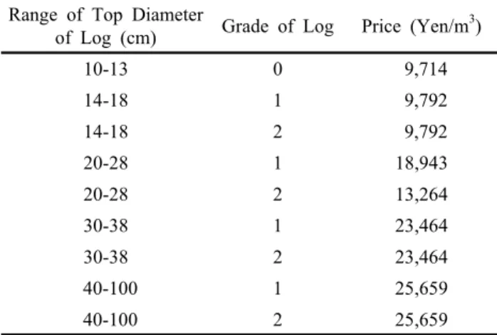
Table 2. Log price as a function of DBH for 4m size log Range of Top Diameter
of Log (cm) Grade of Log Price (Yen/m3)
10-13 0 9,714
14-18 1 9,792
14-18 2 9,792
20-28 1 18,943
20-28 2 13,264
30-38 1 23,464
30-38 2 23,464
40-100 1 25,659
40-100 2 25,659
Note: Grade of log is determined by the position of log produced from a tree. “1” means the 1st log from the bottom of a tree, and the rest is the 2nd grade with small diameter as 0 grade
Fig. 3. NPV of the optimal solution.
ing method (thinning from below, thinning from above, or proportional thinning).
With 1% discount rate and 8,000 yen/m3 for felling costs, we searched for an optimal thinning regime to maxi- mize the net present value of all returns from thinning and final harvesting. Since our optimization model is discrete, we applied 5 trees as an interval of thinning in- tensity and 5 years as an interval of thinning timing in the searching process of DP. The benefits were based on the price of logs produced from trees. We used the price data on log as a function of the top diameter of log at the log auction market in Toyama shown in Table 2. As can be seen from the table, the price changes not only by the top
diameter size, but also by the grade of log determined on the basis of the position of log cut. The H/D ratio was calculated by 100(H / D) by adjusting the dimension of each estimate, where H and D are the average height (m) and DBH (cm) of a forest stand.
We considered two cases for optimization. One was without any H/D ratio requirement, and the other is with the ratio less than or equal to 65% at the thinning and felling periods by
100 ( ) 65
( )
n
n
H m DBH cm
⋅ ≤
(14) Hn : Average height at the n-th stage
DBHn : Average DBH at the n-th stage
The difference in the objective value from these two cases was regarded as a cost induced by the H/D ratio requirement for snow damage protection. Figure 3 shows the optimal net present value over different rotation age under two cases. The gray “x” symbol represents a solu- tion without the H/D ratio requirement, while the black
“x” is with the requirement. From these outcomes, the optimal rotation age turns out to be 65 years for the first case, while 50 year rotation age was for the restricted case. The difference in NPV, CSD, ranged from 179,867 to 1,910,713 yen/ha for the rotation age of 20 to 75 years.
Sudden change was observed for 25 and 30 year rotation.
Under the optimal rotation of 65 years, the cost became 914,226 yen/ha as in Figure 4.
The above difference was calculated based on different
Fig. 4. Difference in NPV.
Table 3. Annual payment under different rotation age Rotation Age Annual Payment(yen/ha/yr)
20 9869
25 85900
30 60385
35 20626
40 15060
45 12102
50 10416
55 10503
60 19075
65 19006
70 17723
75 16758
rotation length, so that the following annual payment was used to compare the results.
1 ( 1 ) 1 1
1 ( )
1
T
SD T r
C AP
r
− +
=
− + (15)
where
CSD : Induced cost for snow damage protection APT : Annual payment
T : Rotation age r : Interest rate (1%)
Table 3 shows the resultant annual payment under different rotation ages. As was observed in Figure 4, annual payment was the largest for the rotation age of 25 years. It ranged from 9,869 yen/ha/yr of the rotation age
20 years to 85,900 yen/ha/yr of the age 25 years. At the optimal rotation age for the restricted case, it was 10,416 at age 50 years. More or less, 10,000 yen/ha/yrto 20,000 yen/ha/yr seemed to cover the payment from the rotation age of 35 to 75 years.
CONCLUSIONS
In this paper, we conducted cost evaluation of the snow damage protection through the optimization framework for the forest stand management of sugi forests. If the induced costs by the snow protection management scheme becomes more than the expected cost of snow damage on the forest management, we would stay with the optimal thinning regime without considering snow damage pro- tection into the management scheme. If not, it would be better off for the forest manager to maintain the optimal regime under the snow protection scheme. In the analysis, we utilized the height-DBH ratio for the management scheme against snow damage for the cost evaluation of snow damage. The previous study indicated that the H/D ratio should be maintained less than or equal to 65%
against snow damage, so that we used this requirement as a constraint into the optimization framework.
Our experimental analyses showed first that the optimal rotation age was 65 years for the unrestricted case, while 50 year rotation age was for the restricted case. The difference in NPV of these two cases as the induced costs ranged from 179,867 to 1,910,713 yen/ha over the rota- tion age of 20 to 75 years. Under the optimal rotation of 65 years, the cost became 914,226 yen/ha. In order to reduce an effect of different length of the rotation age, annual payment was next calculated based on the dif- ference in NPV. The largest was 85,900 yen/ha/yr of the age 25 years, while the smallest was 9,869 yen/ha/yr of the rotation age 20 years. At the optimal rotation age of 50 years for the restricted case, it was 10,416. All in all, 10,000 yen/ha/yr to 20,000 yen/ha/yr seemed to cover the payment from the rotation age of 35 to 75 years.
Although the results indicated here are limited to the
assumed situations, the results suggested that cost evalua- tion through the provided approach is useful for the forest policy toward snow damage protection through the mana- gement scheme. The induced costs can be used as the basis for the coverage of snow damage in the forest mana- gement. The cost for forest owners could be offset by this coverage.
LITERATURE CITED
Adams, D. M., and E. K. AR. 1974. Optimizing the management of unevenaged orest stands. Can. J. Forest Res. 4: 274-287.
Amidon, E. L., and G. S. Akin. 1968. Dynamic programming to determine optimum levels of growing stock. For. Sci. 14: 287- 291.
Arimizu, T. 1958a. Regulation of the cut by dynamic programming.
J. Oper. Res. Soc. Japan 1: 175-182.
Arimizu, T. 1958b. Working group matrix in dynamic model of forest management. J. Jpn. For. Soc. 40(5): 185-190.
Arthaud, G. J., and W. D. Klemperer. 1988. Optimizing high and low thinnings in loblolly pine with dynamic programming. Can.
J. For. Res. 18: 1118-1122.
Brodie, J. D., and R. G. Haight. 1985. Optimization of silvicultural investment for several types of stand projection systems. Can. J.
For. Res. 15: 188-191.
Brodie, J. D., and C. Kao. 1979. Optimizing thinning in Douglas-fir with three descriptor dynamic programming to account for ac- celerated diameter growth. For. Sci. 25(4): 665-672.
Brodie, J. D., Adams, D. M. and C. Kao. 1978. Analysis of economic impacts on thinning and rotation for Douglas-fir, using dynamic programming. For. Sci. 24(4): 513-522.
Chen, C. M., Rose, D. W. and R. A. Leary. 1980. Derivation of optimal stand density over time-a discrete stage, continuous state dynamic programming solution. For. Sci. 26(2): 217-227.
Haight RG, Brodie JD, Dahms WG (1985) A dynamic program- ming algorithm for optimization of lodgepole pine management.
For. Sci. 31(2): 321-330.
Hiller FS, Lieberman GJ (1990) Introduction to operations research.
McGraw-Hill, New York.
Kato A, Nakatani H, Taira H (1992) Relationships of snow damage to stand and topographic factors in sugi stands. J. Jpn. For. Soc.
74(2): 114-119. (In Japanese).
Kato, A. and K. Tanaka. 1997. Parameter estimation for Boka sugi forest stands in the system growth simulato. Chubu Forest Research 45: 43-46 (In Japanese).
Kato, A., Zushi, K. and K. Tanaka. 2008. The growth parameters of the system yield table “Silv-no-mori” in Kawaidani-sugi clone (Cryptomeria japonica D.Don). J. Toyama FFPR Res. Center. 21:
9-16 (In Japanese).
Martin, G. L. and E. K. AR. 1981. A dynamic programming analysis of silvicultural alternatives for red pine plantations in Wisconsin.
Can. J. For. Res. 11: 370-379
Paredes, V. G. L. and J. D. Brodie. 1987. Efficient specification and solution of the evenaged rotation and thinning problem. For.
Sci. 33(1): 14-29.
Riitters, K., Brodie, J. D. and D. W. Hann. 1982. Dynamic program- ming for optimization of timber production and grazing in pon- derosa pine. For. Sci. 28(3): 517-526.
Schreuder, G. F. 1971. The simultaneous determination of optimal thinning schedule and rotation for an even-aged forest. For. Sci.
17(3): 333-339.
Tanaka, K. 1995. A system for prediction a forest stand table and height curve (Silv-Forest). In: Research on development of growth simulators, Konohira, Y. (ed.). pp. 22-32. (In Japanese) Torres-Rojo, J. M. and Brodie, J. D. 1990. Demonstration of benefits
from an optimization approach to the economic analysis of natural pine stands in Central Mexico. Forest Ecol. Manag. 36(2-4): 267- 278.
Valsta, L. T. and J. D. Brodie. 1985. An economic analysis of hard- wood treatment in loblolly pine plantations-a whole rotation dyna- mic programming approach. In: The 1985 symposium on system analysis in forest resources, Dress PE, Field RC (eds.). Georgia Center for Continuing Education, Athens, pp. 201-214.
Vonesh, E. V. and R. L. Carter. 1987. Efficient inference for random- coefficient growth curve models with unbalanced data. Biometrics 43: 617-628.
Yoshimoto, A. and R. Marušák. 2007. Evaluation of carbon seque- stration and thinning regimes within the optimization framework for forest stand management. Eur. J. For. Res. 126(2): 315-329.
Yoshimoto, A., Paredes, V. G. L. and J. D. Brodie. 1988. Efficient optimization of an individual tree growth model. In: The 1988 symposium on systems analysis in forest resources, Kent BM, Davis LS (eds.). USDA Forest Service. General Technical Report RM-161, pp. 154-162.