대체 에너지의 다중레벨 모델링과 시뮬레이션
Multi-level Modeling and Simulation for Sustainable Energy
P. J. van Duijsen*, 오 용 택**
P. J. van Duijsen*, Yong-Taek Oh**
요 약
녹색에너지의 모델링과 시뮬레이션은 연구하고자 하는 시스템의 형태에 따라 크게 의존한다. 모델링과 시뮬레 이션의 주요내용은 반도체 물리(태양전지), 전기모터/발전기(풍력터빈), 전형적인 제어전략에 의한 전력전자(계통연 계)등 매우 다양하다. 이들 기술들을 정확하게 모델링하는 것은 다양한 시뮬레이션 기술과 많은 모델들을 필요로 한다. 시뮬레이션을 더욱 정확하게 혹은 상세하게 하기 위해서 모델링은 특정레벨 즉, 시스템, 회로, 요소 레벨 등 으로 수행하여야 한다. 다양한 레벨의 조합은 모델 방정식과 이용 가능한 매개변수들에 대한 전체적인 모델의 유 용성을 크게 개선할 수 있다.
Key Words : Modeling, Simulation, Wind, Solar, Induction Generator, MPP, eMobility ABSTRACT
Modeling and simulation for Green Energy depends largely on the type of system under investigation. The topics are very wide ranging from semiconductor physics (solar), electrical motor/generator (wind turbines), power electronics (grid connections) to typical control strategies. To correctly model these technologies requires a broad set of models and various simulation techniques.
To further refine or detail the simulation the modeling has to be performed on a specific level, being system, circuit or component level. Combinations of several levels allows gradually improving the validity of the overall model against available parameters and model equations.
* Technical University of Delft ([email protected])
** Korea University of Technology and Education ([email protected]) 제1저자 (First Author) : P. J. van Duijsen
교신저자 : 오용택 접수일자:2011년 4월 27일 수정일자:2011년 6월 08일 확정일자:2011년 6월 19일
I. INTRODUCTION
The market for green and renewable energy is growing, but also presents numerous new challenges when it comes to technology, environment and acceptance. Concerning technology, these challenges require not only new ideas, but also engineering effort to realize these new technologies. Reduction of cost and improving system efficiency are the two main engineering challenges.
Currently, wind and solar energy generation are the most important renewable energy generation methods. Electric and hybrid vehicles are considered the most important research area in the field of worldwide energy mobile consumption. In order to be mobile, energy produced by wind and solar technologies has to be stored for later mobile use.
The traditional build and test approaches are both time-consuming and expensive. Also building and testing does not provide enough insight to reach an optimal design, not even thinking about the costs and construction time.
Use of engineering simulation software like Caspoc [10] helps with the optimization of entire designs, whether it is a small-scale solar project or a large offshore wind park. Detailed testing in simulation is required to ensure the conformity to a wide range of requirements [1]. On the other hand, the simulation gives valuable insight into the behavior of the system under investigation and allows studying phenomena that are visible in simulation, but are hard to measure in a real set up. Therefore simulation and animation are viable tools, not only for the engineer, but also for education [2]. Especially the animation feature allows for a better visual insight and understanding in complex systems.
II. Variety of Technology
Research for modeling and simulation in the field of green and renewable energy is a broad topic. Not only the systems are very diverse, like wind and solar, but also the physical background of each type of green energy system varies greatly. For the modeling and simulation, this leads to two observations that have to be taken into consideration:
1) Physical background of the underlying system
2) System or detailed of the model of systems under investigation
First, for example, wind energy requires knowledge on electromagnetic energy conversion, while solar requires knowledge on semiconductor devices. Control in solar systems is mostly a sort of a smart search algorithm that finds the optimum electric load for a solar module, while in wind power systems, the control is clearly dependent on the wind speed. Fuel cell, reformers and batteries require knowledge of chemical processes. So generally speaking various technologies are used when working with green energy systems.
Second the components can de modeled as simple system blocks with clearly defined functions, but on the other hand multilevel models including all details can model them. For example, generator modeling in FEM and detailed semiconductor models in solar modules.
III. Levels of Modeling
Instead of setting up models just based on existing models available in a standard simulation package, it is better to have a better understand in the levels of modeling. Depending on the required details in the simulation results and the availability of model parameters, various models are possible. In general there is a division among
three levels of modeling. There is a general system level model, a more detailed circuit level model and finally a very detailed component level.
Each level can contain linear and non-linear model-equations and the complexity might vary between the levels, the overall issue is that the fidelity of the model gets higher at a higher modeling level. For example, the detailed component model requires more parameters that an overall system model and also the simulation results will include small details that belong to the solution of the detailed equations inside the detailed component model. A system level model might be very complex and yield a highly non-linear equation. But as long as the inside details compared to the component model are negligible, the simulation results will be much more simple compared to those from a more detailed component level simulation.
The first step is to get an overall picture of the power distribution in the system and to look at the load of every single system component.
Typically idealized system components are used.
On this system level an early concept of the control system can be designed and tested in simulation. For example, the Maximum Power Point (MPP) control method can be tested together with the solar module, DC converter and grid connection. Another example is the overall energy harvesting of a grid connected wind turbine for varying wind speed. [3]
The second step is to look at each component more in detail on the second, the circuit level. One method is to replace the idealized system models with more detailed models. This increases overall simulation time, but gives more detailed simulation results. For example, a model including the semiconductor switches (IGBT, Mosfet and diodes) could replace the ideal continuous model of a grid-connected inverter [4]. The simulation results would now also include harmonics as well as typical modulation influences.
The third step would be to look at each component more in detail on the third, the component level. Instead of using more detailed lumped circuit models with limited parameter sets from the second step, the models could be based on more detailed engineering software. For example, a non-linear model replaces the three-phase generator circuit model, where the input-output relations are pre calculated in Finite/Boundary Element Method (FEM/BEM) software.
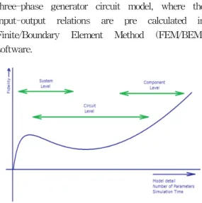
Fig. 1. Fidelity of model
The advantage of modeling on various levels in Caspoc is the gain in simulation speed when using system models and the matter of details in component simulations. On the circuit level, the interaction between the various components can be studied more in detail as with a system simulation, but still requires less simulation time compared to the simulation on the component level.
Figure 1 shows the dependency of the fidelity on the detail of the model and the availability of parameters. At first the fidelity is rising fast. At a certain moment, increasing the model does not seem to be an improvement any more, as the model gets very complex and the interaction between the components becomes prone. After further increase of model detail, the fidelity increases again, and keeps on increasing for every additional model extension. The system level can be viewed as the most left part of this
characteristic, while the middle part covers the circuit level and the most right part the component level.
Level Wind turbine Generator Inverter
System Level P = ½ρACpω3 u∙i = T∙ω
uin ∙ iin
=
uout ∙iout
fin ≠ fout
Circuit Level
Additional aero-elastic
and aero-dynamics
Cp(l,pitch)
dq model Sinusoidal
back-emf
Switched level model
PWM / SVM PQ control
Component Level
Additional dynamics of the drive train
such as shaft-stiffnes
and blade-inertia
FEM model Back-emf
includes harmonics Influence of
saturation
Parasitic inductance
Mosfet / IGBT switching
delay Temperature dependency Table 1. Modeling levels for the wind power system from figure
To get a better insight in the variety of the modeling levels, the wind power generation system from figure 2 will be used as an example.
Each part of the system is shown in table 1, where depending on the level of modeling, the level of modeling is explained.
Fig. 2. Simplified architecture of a wind power system
As can be seen from table I, every single part of the system from figure 2 can be modeled on various levels. As long as the input output ports of each part remain equal, these parts can be combined into a single model. For example the
input of the wind turbine is the wind speed, while the output is the rotating shaft. This shaft is then connected to the shaft of the generator that has a three phase electrical connection on the left side.
The inverter has a three phase electrical connection on the left as well on the right side.
This makes the interconnection of, for example, a system level wind turbine model with a circuit level three-phase generator model with a component level model of the inverter possible.
This arrangement would be useful for studying the transients inside the inverter for various wind turbine power/speed combinations. On the other hand, a circuit level wind turbine connected to a system level generator and inverter would show the influence of various wind speeds on the amount of power generated.
Ⅳ. PV Generation Modeling
1. Solar Module Modeling
Let’s have a look at a number of typical simulation studies that give insight in the system.
We start with a simple model for the a single solar cell and is shown in figure 3.
Solar Cell Load Resistance
I solar
Fig. 3. Solar Cell model with resistive load
Here each solar cell is modeled using a sunlight dependent current source and a parallel diode. And yes, the diode is drawn in the correct direction. If the voltage across the solar cell gets beyond the typical on-state diode voltage of around 0.6-0.7 volts, the diode starts conducting and short circuits the solar cell current. A load resistor is added to the model in figure 3, to test the solar cell model in a simulation. This circuit level model is still without losses. A series and a parallel resistance mostly model these losses.
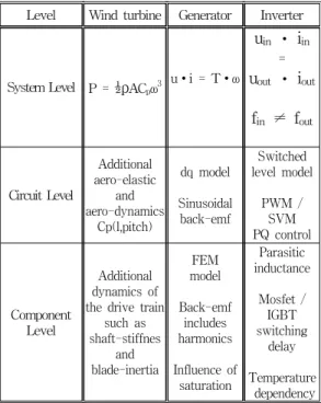
The single solar cell model is used in a solar module containing 4×2 cells, that for some reason is partly shaded. This is simulated on the second level (circuit level), since we want to know how the shading influences the behavior of the solar module. A circuit level model is shown in figure 4. In this model the intensity of the current is indicated by the color, red is maximum current and black is zero current. The shaded cell current is zero and this shaded cell blocks the current from the other cells that are in series with the shaded cell. The values for the solar and shading current are controlled manually by the ‘updown’
blocks in the model. In Caspoc, the user can control these currents and see the current distribution inside the module. A load resistor that is also manually controlled by an ‘updown’ block sets the operation point of the solar module.
Shading one cell means turning off a complete column in a module and therefore bypass diodes are included. However, bypass diodes also reduce the efficiency, while increasing the costs of the solar module. In the module in figure 4 the bypass diodes are omitted for the sake of simplicity.
In the simulation it becomes visible how the current distribution is inside the module. The solar cells that are in direct sunlight produce around 3A. Part of this current flows through the anti-parallel diode. All solar cell in the left column of the module produce 3 amperes and this current flows via the series resistance’s R1, R4, R10 and R12 to the load resistance. The shaded cell produces only 1 amperes and this means that the current (3 amperes) produced by the other cells in the right column, cannot flow through that shaded cell. Therefore the current from each cell in series with the shaded cell will flow through the anti-parallel diode. The total current in the right column is therefore limited to 4 amperes. Since the load resistance is set to a low value, the maximum short-circuit current flows through the load resistance.
SHADED UPDOWN
1
= 4.027
= 8.055n 1n
R17 1n A3 D3 R5 100 R6 50m
A4 D4 R7 100 R8 50m UPDOWN
3
A1 D1 R3 100 R1 50m
A2 D2 R2 100 R4 50m
A5 D5 R9 100 R10 50m
R12 50m
A7 D7 R13 100 R14 50m
R16 50m Ishade
Ishade
ii u
i R
u
Isolar
Isolar Isolar
Isolar
Isolar
Isolar
Isolar Isolar
1 1
4.027 8.055n
4.027 1n
8.055n[Volt]
3
3 3
3
3
3
Fig. 4. Shading and current distribution inside the solar module
If bypass diodes would be included in the solar module, the current from the solar cells in direct sunlight would be flowing through the bypass diodes and thereby making the maximum current equal to 6 Amperes.
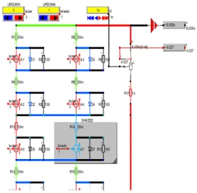
2. Grid Connect Solar converter with MPP The second example shows the control of a grid-connected solar system. Figure 5 shows the circuit model including the MPP control and grid-connection control.
A detailed second level circuit model that includes load dependent loss and temperature dependency models the solar module. A boost converter that regulates the MPP for the solar module electrically loads the solar module. The boost converter is also modeled as a second level circuit model. The MPP controller is a first level system model that calculates the derivative of the power as a function of the voltage of the solar module. Together with the first level system model for the PI controller, the amount of power harvested by the solar module is maximized. The last part is the grid connection. Here a first level system model for the inverter and control is used.
This simulation shows the mixture between the various levels in modeling.
Fig. 5. Solar module with boost converter, grid connection and MPP control Since all models are connected in a circuit level
model, the u-i interactions can be studied as well as the MPP control part.
The single-phase grid converter is a very simple system level model that only controls the current delivered to the single-phase grid. In a more detailed study, the complete single-phase inverter with controlling algorithm and modulation strategy as well as grid synchronization could be applied. However for studying the behavior of the MPP controller, this simplified system level model suffices.
Scope 1 in the Caspoc simulation in figure 5, shows the u-i characteristic of the solar module.
Small circles indicate the characteristic, while the arrow points to the current point of operation.
Scope 2 shows the grid-side current, which is in phase with the grid voltage. Scope 6 shows the amount of power delivered by the solar module
and the amount of power delivered to the grid.
Ⅴ. Wind Power Modeling
1. Induction Generator
In the next example a more detailed model of a generator for a wind power system is examined.
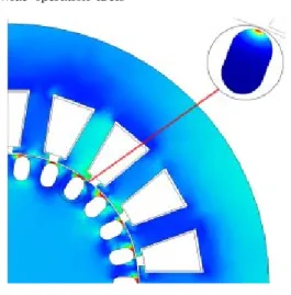
The efficiency of a wind power generator has to be optimized for two main reasons. First to maximize the amount of power the wind turbine generator can deliver and secondly to reduce to reduce the losses inside the generator. Each reduction of loss in the generator means that the generator delivers more output. Even 1% efficiency improvement is important when thinking about an average off-the-shelf 2 Megawatt generator. An improvement of 1% means a reduction of 20kW of loss that not has to be cooled (also consuming extra power). So the bottom line in generator design is to optimize the generator efficiency over
Fig. 6. Field magnitude plot in the rotor and stator of an induction motor; current density induced in one rotor bar (inset)
a wide operation area.
Specialized FEM software that can model the generator in detail with manufacturer data for magnetic and ferromagnetic material is used here.
Especially Boundary Element Method [BEM]
solvers are in applicable [5], since they do not require meshing of the airgap and therefore are more accurate than only FEM solvers. In BEM, only the outer surface has to be defined and no mesh in the airgap and exterior space is required.
More details about BEM/FEM can be found in [5].
From the BEM/FEM simulation, look-up tables are generated that can be used in the system level or circuit level simulations. Figure 6 shows the current distribution inside a rotor bar of an induction generator. Depending on the slip of the generator, the current distribution varies and thereby also the losses inside the rotor. Secondly because of the skin effect that causes this current distribution in the rotor winding, also the rotor winding parameters, especially the leakage component parameters vary. These parameters have a sincere impact on the control of the motor/generator and on the component level they have to be calculated in detail.
2. Wind Turbine Maximum Power Control The second wind energy example shows an
overall system simulation of a wind power system.
A more detailed second level circuit model can replace every single component in this first level system simulation. In this example, only the wind speed to rotor angular speed ratio (tip speed ratio [TSR], λ) is modeled in a circuit level model.
Also third level component models or even a mix between first, second and third level models would be possible in this type of simulations.
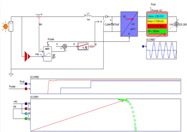
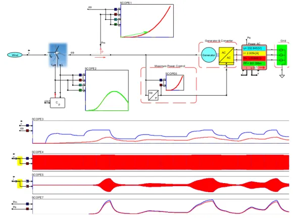
Figure 7 shows a grid connected wind turbine system with optimum power control, modeled in Caspoc. The maximum amount of power a wind turbine can deliver is equal to κω3. Therefore the control electrically loads the wind turbine generator such, that it subtracts exactly κω3 Watts from the wind turbine and thus keep the system in equilibrium. For varying wind speed, the control directly adjusts the amount of power drawn from the wind turbine generator and also controls the amount of power delivered into the main grid. A second level circuit model models the wind turbine, where the ratio between the wind tip speed and rotor angular speed determines the amount of power the wind turbine can deliver.
This model is a minimum requirement when investigating the behavior for varying wind speed.
The generator is modeled as a first level system model, as the primary goal is to study the stability of the overall control system. The wind turbine includes the TSR dependent power coefficient Cp(λ, β), where λ is the TSR and β is the pitch angle of the rotor blades. The characteristic of Cp(λ, β) is shown in scope 2 in figure 7 and this curve can be specified either by analytical equations, or by a look-up table from measurement results. The amount of mechanical power Pm is displayed in scope 1 as function of the angular rotor speed. Inside the “Maximum Power Control”, the electrical power is calculated and controls the combined system level Generator/Inverter model. The left side of this model is the shaft of the generator, while the right side is the electrical connection to the grid.
The remaining scopes in figure 7 show from top
Grid Gener ator & Converter
Maximum Power Control
Gener ator AC Wind AC
pitch C
p
Power AC
3@
i u
SCOPE2
SCOPE3
SCOPE1
SCOPE4
SCOPE5
SCOPE7
@ P
SCOPE6
i= 2.005k [A]
u= 232.845 [V]
P= 1.332MEG [W]PF= 951.056m
@
v
Pm
@
Pe
v
@
u
Pm Pe i
u i
Fig. 7. Wind turbine system with optimum power control
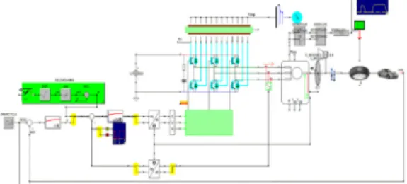
Fig. 8. Hybrid Power Drive Train to bottom, wind speed and angular shaft speed,
grid-side voltage and current, mechanical and electrical power. The scopes clearly show the dependency of the amount of power delivered to the grid on the wind speed.
Ⅵ. Wind Power Modeling
Electric Mobility is an emerging technology simply because fossil resources are shorter every day. Electric vehicles are the key for future transportation, keeping in mind that fossil liquid fuel resources soon to be exhausted. The main advantage of liquid fuel is the high energy density compared to other portable energy storage mediums.
For example, 5 liters of petrol gets you 100km by car, but driving a car with a fully loaded battery of only 5kg, will not get you very far.
The driving range of electric vehicles is the main concern in regarding electric mobility. The range
requirement is the overall efficiency and weight optimization in a new design. The hybrid vehicle is seen as a possible option to overcome the range limits, but this is only a temporarily technology as it consists of two different technologies, where one is based on fossil fuel resources. From the viewpoint of price, having both an internal combustion engine and an electric motor on board, the benefit of a hybrid seems to be arguable.
Fig. 9. Field oriented control of an electrical drive train.
Figure 8 shows the electrical and mechanical drive train of a hybrid car [8], including combustion engine, electric motor, planetary gear and wheels. The models in figure 8 are all on the circuit level. Also the mechanical drive train is modeled in Caspoc on the circuit level, as the rotational components are modeled in the same way as the electric circuit is modeled. Here angular speed and torque replace voltage and current.
1. Power Electronics and Thermal Model To refine the model of the hybrid vehicle, the electrical drive train is modeled again in figure 9.
Here a field oriented control, permanent magnet synchronous machine and power electronics is modeled on the mixed circuit/component level.
[6][7][8]
A virtual driver is included to test the model against a given time-speed characteristic. Since also the inverter components are modeled in detail including the loss calculation, allowing the thermal behavior of the power electronics to be studied in detail. The virtual driver controls the field-oriented controller, that using space vector modulation controls the power electronics inverter. Space vector modulation is required here, as the harmonics generated by this type of modulation both influence the losses in the power electronics and electrical machine as well the dynamic behavior of the electrical machine. [9]
Ⅶ. Conclusions
Multilevel modeling allows the combination of various levels of models to be interconnected.
Depending on the required simulation models system models can be employed for overall system behavior and can be interconnected with detailed component models. Concentrating on the minimum required levels in a model reduces overall simulation time and does not overcomplicate the total model.
Acknowledgements
"This paper was partially supported by the education and research promotion program of KUT"
References
[1] Bauer, P & Duijsen, PJ van (2005).
Challenges and advances in simulation. In s.n. (Ed.), Proceedings of the 36th power electronics specialists conference (pp.
1030-1036). Piscataway, USA: IEEE.
[2] Bauer, P & Duijsen, PJ van (2008). Power electronics simulations. International review on computers and software (IRECOS), 3(3), 307-314.
[3] Duijsen, P van, Bauer, P & Chen, F (2006).
Modeling and simulation for wind energy. In s.n. (Ed.), Proceedings of the Taiwan power electronics conference & exhibition (pp.
1087-1092). Taipei: Taiwan Power Electronic Association/IEEE Taipei Chapter.
[4] Bauer, P & Duijsen, PJ van (2009).
Simulating losses and semiconductor junction temperature in power electronics.
Bodo's power systems, 9, 36-38.
[5] B. Klimpke; A Hybrid Magnetic Field Solver Using a Combined Finite Element/Boundary Element Field Solver;
Sensors Magazine; May 2004
[6] van Duijsen, P.; Leuchter, J.; Bauer, P.;
2.5×3.0㎜
삽입그림으로 2.5×3.0㎜
삽입그림으로 Lifetime estimation with thermal models of
semiconductors; Energy Conversion Congress and Exposition (ECCE), 2010 IEEE; pp 978 - 985
[7] Duijsen, PJ van, Bauer, P & Leuchter, J (2010). Thermal models for semiconductors.
In S Mircevski & D Boroyevich (Eds.), 2010 14th International Power Electronics and Motion Control Conference (pp. 23-28).
Ohrid, Macedonia: IEEE.
[8] Bauer, P & Duijsen, PJ van (2009).
Sensorless control for electrical and hybrid electric vehicles. Bodo's power systems, 11, 50-52.
[9] Chao, D.C.-H.; van Duijsen, P.J.; Hwang, J.J.; Chin-Wen Liao; Modeling of a Taiwan fuel cell powered scooter; International Conference on Power Electronics and Drive Systems, 2009. PEDS 2009. , pp: 913 – 919 [10] Caspoc, Simulation Research, www.caspoc.com
Peter van Duijsen
Peter van Duijsen received the his M.Sc. and Ph.D. degree from the Technical University of Delft, the Nethelands, in 1989 and 2003, respectively.
He founded the company Simulation Research in 1989 where he is currently heading the research and development department. His research interests include power electronics, electrical drives and renewable energy simulations.
오 용 택 (Yong-Taek Oh)
Yong-Taek Oh received his B.S degree from the Sungsil University, Korea in 1980.
He received M.Sc and Ph.D degree Electrical Engineering from the Yonsei University, Korea in 1982 and 1987 respectively. From 1987 to 1991, He was with the computer Center of Korea Electrical Power Corporation as a Section Chief.
He joined the faculty of Korea University of Technology and Education, Cheonan, Korea in 1991 where he is currently a professor in the school of Electrical Engineering.
His areas of research interest are power system analysis, computational application in power engineering included simulation and modelling.