Unsupervised feature learning for classification

한국컴퓨터정보학회 하계학술대회 논문집 제24권 제2호 (2016. 7)

51

Unsupervised feature learning for classification

Mamur Abdullaev ^O , Jumabek Alikhanov ^* , Seunghyun Ko ^* , Geun Sik Jo ^*

O* Department of Computer and Infomation Engineering, Inha University

e-mail: [email protected] ^O , [email protected] ^* , [email protected] ^* , [email protected] ^*

●

●

In computer vision especially in image processing, it has become popular to apply deep convolutional networks for supervised learning. Convolutional networks have shown a state of the art results in classification, object recognition, detection as well as semantic segmentation. However, supervised learning has two major disadvantages. One is it requires huge amount of labeled data to get high accuracy, the second one is to train so much data takes quite a bit long time. On the other hand, unsupervised learning can handle these problems more cheaper way. In this paper we show efficient way to learn features for classification in an unsupervised way. The network trained layer-wise, used backpropagation and our network learns features from unlabeled data. Our approach shows better results on Caltech-256 and STL-10 dataset.

키워드: CNN, Unsupervised learning, zoom-out dataset

I. Introduction

In the last few years Convolutional Neural Networks(CNN) that trained with massive amounts of labeled data in a supervised way, have shown a state of the art performances in semantic segmentation [1, 2, 3], detection [4, 5], classification [6, 7, 8].

However, labeling data is tedious work and requires much time to label it. For example, ImageNet has 1.3 million images.

It took hundreds of hours and human effort to label them. When only unlabeled or a limited number of labeled data available, supervised learning algorithms does not work. In such cases unsupervised or self-learning comes handy.

Useful features can be learned from unlabeled data with some unsupervised learning algorithms such as Autoencoders, Sparse Autoencoders, and Restricted Boltzmann Machine (RBM).

Autoencoders has three layers (input, hidden, output) fully connected each other. It takes an image as an input and its target also the same image in the output layer. It is machine learning tool that learns features from image (input layer) discriminating (hidden layer) and comparing (output layer) with itself. In our work we use deep Convolutional Networks to learn

features from unlabeled data and applying them for classification. We also show that our tested result in two datasets get better classification result than pervious works.

II. Related Work

Our work is closely related to [9] work. In this work authors made new dataset from unlabeled images, dividing an image into some patches and get the patches which contain object or part of objects. Then augmented transformed these patches in some ways like changing color, scale and rotation in order to make them robust to noises. Every sample is given as a class label for its subsamples. They call it Exemplar-dataset.

For training they used three convolutional layers and one fully connected layer. In our work, we transform images following their transform way, but making dataset from image patches and our architecture are differ in many ways. We named out dataset zoom-out dataset.

There are some more works [10, 11, 12] used k-means algorithm to learn filters later use it for classification. Because k-means clustering can be used as a fast alternative training method.

On the other hand, employing this method in practice is not completely trivial. In [12] they clustered image patches before giving them as an input and every cluster point is given as a class label for the group images.

In our work can be separated into two parts: a feature extractor and a classifier. An unsupervised term refers to feature extractor part while our approach learns features from unlabeled data.

The output of feature extractor (learned filters from unlabeled data) is given to classifier like already trained model (also

한국컴퓨터정보학회 하계학술대회 논문집 제24권 제2호 (2016. 7)

52

descriptor). To be concrete, when we train dataset in supervised manner we use the filter which we get from feature extractor rather than using random filters.

In the following section, explained how to make zoom-out dataset and our proposed architecture to train network.

III. Feature learning

3.1 Creating zoom-out Training Data

Surrogate dataset is well explained and tested in [9]. Before [9] work data augmentation approaches used only one patch to make a class label. But the authors of the paper [9] transform one patch into randomly selected transformations and make between 50 and 150 samples per class.

Our approach is similar to [9], but we are considering every patch having individual as well as shared features rather than taking only patches which contain object or part of objects.

The work is start by dividing a random image into small patches.

These patches will be class label for their sub-patches. The small patches also divided into more smaller patches. The main idea of doing this is to learn invariant features between same classes and discriminative features between different classes.

In order to be one class’s instance, sub-patches should have two components. 1) There must be at least one feature that is similar for images of the same category 2) There must be at least one feature that is sufficiently different for patches of different categories.

Our experiments held on two datasets which are Caltech-256 and STL-10. Caltech-256 has 256 classes, 80-120 images in each class. The images are different size. STL-10 dataset has 10 class, total 5000 training and 8000 test images. The image sizes are 96x96 pixel.

First Caltech-256 dataset is resized images 256x256 and divided them into 128x128 patches with a stride of 32 pixels. It will give us 25 sub-patches. Then these sub-patches divided by 64x64 with a stride of 32 pixels, more smaller patches. Finally, applied a few augmentations: left-right mirroring, rotations of 20 degree and changing HSV color parameters. For STL-10 dataset also same steps applied. They are resized 112x112, divided by 48 with stride of 32, these sub-patches divided by 24 with a stride of 8. Before training all patches resized, Caltech-256 to 64x64 and STL-10 32x32.

Stride is chosen 1/3 of a patch size and it is 1/2 of small patch because in that case any patch’s 1/3 part is learned as an only instance of one category, 2/3 part is learned as an instance of two and three (shared features between two or three classes) category. We experimented different strides but strides explained

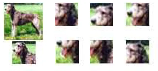
above have shown better results in both datasets. Figure 1 shows one example of STL-10 dataset. It is named zoom-out dataset, because every feature is learned in three patches and deferent scales.

Figure 1. Left top is the original image, left bottom is one patch of original image, It gives 9 patches like this in one image (also class label), and the other images are instances of the patch

(sub-patches). It will leave us 9 sub-patches in per patch.

Overall one image divided by 81 patches.

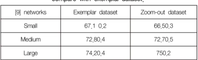
Our zoom-out training dataset is tested with [9] network to compare with exemplar training dataset. Table 1 shows results tested on STL-10 dataset. The small network has 2 convolutional and one fully connected. The medium and large networks have 3 convolutional and one fully connected layers.

3.2 Proposed Architecture.

Our approach for generating dataset(zoom-out) performs better than exemplar dataset when we test in [9] networks, we build our network to increase accuracy even better.

Autoencoder, sparse aoutoencoder, Restricted Boltzmann machine have been widely used as a feature extractor. They usually have three layers which are encoder (input), hidden and decoder (output). Because these layers fully connected they take much time to train. But [9] and [12] show that convolutional networks can learn useful features. The network learn some part of an input image in the first layer, calculate its activation, max pool to reduce the feature map dimension and send the feature map as an input to next layer. It is computationally cheap comparing to cully connected networks.

Our networks different for STL-10 and Caltech-256 dataset because, two dataset patches are resized to different size. By resizing STL-10 images and network depth two times smaller than Caltech-256 images and depth

한국컴퓨터정보학회 하계학술대회 논문집 제24권 제2호 (2016. 7)

53

compare with exemplar-dataset.

[9] networks Exemplar dataset Zoom-out dataset

Small 67.1 0.2 66.50.3

Medium 72.80.4 72.70.5

Large 74.20.4 750.2

Our networks are differ from each other in terms of number of layers used. Caltech-256 with 8 layer network 5 convolutional and 3 fully connected layers. STL-10 network has 3 convolutional and 2 fully connected layers. Batch normalization [13] applied for classification, achieved lower error rate. While our networks layers connected in supervised way, we used batch normalization to normalize every batch in convolutional layers. It lead us to get better results and reduce training time. Max pooling layer used to reduce the dimensions of feature maps. Both of the networks all convolutional layers used same kernel with different strides. The same kernel size and strides used in two networks all pooling layers. Our networks trained suing Stochastic Gradient Descent (SGD) via backpropagation manner with caffe framework. We tested other solvers also like AdamSolver in caffe framework but it did not give expected results.

Training started learning rate of 0.001 and momentum is fixed 0.9. While learning feature, used small number of images randomly chosen between 50 and 120. Used number of classes are between 195 and 900, number of patches in each class is 17-30. For our all experiments NVidia tesla 40c GPU.

3.3 Learning Algorithm

Given all transformed patches and sub-patches as an input and declared patches as a target label. The loss between input sample and target is calculated in the following equation









∈ 



∈



   

  



Softmax classifier is used in final layer to distinguish one patch form another and iteratively using backpropagation to minimize the loss over the samples. We did not experiment SVM classifier because [9] and [12] results show it does not give higher accuracy as softmax classifier.

Table 2 shows results that we get by training on zoom-out dataset with our proposed network. It gave same accuracy as we get using [9] network on STL-10 dataset. This is because our small network quite similar to [9] network. But there is 3% increase on Caltech-256. For STL-10 used small network and Caltech-256 used large network.

Table 2. Comparison classification accuracies on two datasets.

Ex-CNN’s large networks result is shown

Algorithms STL-10 Caltech-256

[10] 680.6

[12] 74.1

Ex-CNN 74.20.4 53.60.2

Ours 750.2 56.20.4

Training is stopped when training loss keeps unchanged

IV. Conclusion.

In this work we proposed learning features from unlabeled data for supervised classification. Madden surrogate dataset by dividing unlabeled images into patches and transform them into some other forms. Which helps for network to learn robust filters. Our approach shows better performance on two datasets STL-10 and Caltech-256. Besides we also showed deep neural network can be used to learn features for unsupervised learning while many researches use small number of layers for this task.

Furthermore this work can be improved by filtering input data before training, like using k-means training and clustering patches in to specific groups. We will leave this in our future work

References

[1] ”Fully connected Networks for Semantic Segmentation” J. Long, E. Shelhamer, T. Darrell [2] ”Semantic Image Segmentation with Deep

Convolutional Nets and Fully Connected CRFs”

L.Ch. Chen, G Papandreou, I Kokkinos, K Murphy, Alan L. Yuille.’

[3] Conditional Random Fields as Recurrent Neural Networks”. Sh. Zheng, S. Jayasumana, B.

Romera-Paredes, V. Vineet, Z. Su, D. Du, Chang Huang, and Philip H.S. Torr.

[4] ”OverFeat: Integrated recognition, localization and detection using convolutional networks.” P.

Sermanet, D. Eigen, X. Zhang, M.Mathieu, R.Fergus and Y. LeCun, in ICLR, 2014.

[5] ”Rich feature hierarchies for accurate object detection and semantic segmentation” R. Girshick, J. Donahue, T. Darrell, and J. Malik, in CVPR, 2014

[6] ”ImageNet classification with deep convolutional

한국컴퓨터정보학회 하계학술대회 논문집 제24권 제2호 (2016. 7)

54

neural networks”A. Krizhevsky, I. Sutskever, and G. E. Hinton, in NIPS, 2012,

[7] ”Very deep convolutional networks for large image scale image recognition” K. Simonyan, A.

Zisserman

[8] ”Going Deeper with Convolutions” Ch. Szegedy, W.Liu, Y. Jia, P.Sermanet, S.Reed, D.Anguelov, D.Erhan, V.Vanhoucke, .Rabinovich

[9] ”Discriminative Unsupervised Feature Learning with Exemplar Convolutional Neural Networks”

A.Dosovitskiy, P.Fischer, J.T.Springenberg, M.Riedmiller, T.Brox

[10] “Convolutional clustering for unsupervised learning”

A.Dundar, J.Jin, and E.Culurciello

[11] “Learning Feature Representations with K-means”

Adam Coates and Andrew Y. Ng

[12] “Committees of deep feedforward networks trained with few data” B.Miclut, T.K aster, T.Martinetz, and E.Barth

[13] ”Batch Normalization: Accelerating Deep Network Training by Reducing Internal Covariate Shift” S.

Ioffe, Ch. Szegedy

[14] ”Caffe: Convolutional Architecture for Fast Feature Embedding” Y.Jia, E.Shelhamer, J.Donahue, S.Karayev, J.Long, R.Girshick, S.Guadarrama, T.Darrell