The Method to Setup the Path Loss Model
by the Partial Interval Analysis in the Cellular Band
Kyung-tae Park*, Sung-hyuk Bae**
There are the free space model, the direct-path and ground reflected model, Egli model, Okumura-Hata model in the representative propagational models. The measured results at the area of PNG area were used as the experimental data in this paper. The new proposed partial interval analysis method is applied on the measured propagation data in the cellular band. The interval for the analysis is divided from the entire 30 Km distance to 5 Km, and next to 1 Km. The best-fit propagation models are chosen on all partial intervals. The means and standard deviations are calculated for the differences between the measured data and all partial interval models. By using the 5 Km- or 1 Km- partial interval analysis, the standard deviation between the measured data and the partial propagation models was improved more than 1.7 dB.
Keywords: Path Loss, Cellular Band, Partial Analysis, Propagation Model, Base Station
From the 1990s, many remarkable progresses have been made in the mobile communication systems through AMPS, GSM, and CDMA systems. Currently, the high-speed mobile data services of Wi-Fi, LTE... are available. The expensive fees have been imposed on the cellular system due to the frequency-band allocation. Nevertheless, the analysis on the frequency channel characteristics are not sufficient[1].
The researches on the propagation models in the cellular bands (850MHz) have begun with the wide-use of the mobile phones.
There are the free space model, the direct-path and ground reflected model, Egli model, Okumura-Hata model in the representative propagational models.
The measured results at the area of PNG in Russia were used as the experimental data in this paper. To characterize the n ew propagation model for the PNG area using many conventional propagation models, the measurement data was divided into a number of analysis intervals. Among the conventional propagation ones, the closest propagation model to the measurement data was chosen for each interval. The new propagation model can be assembled from the closest ones. By applying the assembled propagation model to the measurement data in Russia, an improved result on the standard deviation of at least 1.7 dB was obtained.
In article II, the propagation theory and the propagation
* Department of Electronics and Communications Engineering, Masan University
** Masan University (corresponding author) 투고 일자 : 2012. 12. 12 수정완료일자 : 2013. 4. 25 게재확정일자 : 2013. 4. 30
environment in the measured area were introduced. In article III, the measured data in Russia was plotted to graphs, and the method of the partial analysis was proposed. In article IV, the results of the partial analysis were summarized.
In the basic theoretical and conventional propagation models for the cellular system, there are the free-space path loss model, a direct wave and the ground reflected wave model, Egli model, and Okumura-Hata propagation model.
1. The Free-Space Propagation Model
The free space is an air media without obstacles. In figure 1, the free-space path loss can be calculated as follows. The transmitted power which is radiated from a certain source is getting smaller in proportion to the square of the distance between the transmitter and receiver antennas, and then arrives at the effective area of the receiver antenna. The ratio of the received power relative to the transmitted power is the free-space path loss[2].
Fig. 1 The Free-Space Propagation Model[2]
The free-space path loss in the figure 1 is calculated as follows:
Wr
Wt =G tG r( 4πλd )2 (1)
When equation (1) is expressed in decibels,
log log
log log
(2)
can be obtained. Where Wt is the transmitted power, Wr is the received power, Gt is the transmitter antenna gain, Gr is the receiver antenna gain, λ is the wavelength of the radio wave, d is the distance between the transmitter and receiver antennas.
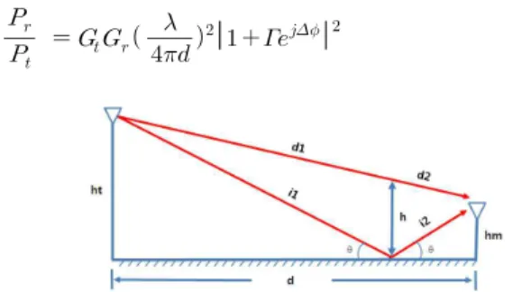
2. The direct wave and ground-reflected wave model The radio wave from the transmitter antenna to the receiver antenna is consisted of the direct wave and ground-reflected wave as in figure 2. The final received power at the receiver antenna is the sum of the direct wave and the reflected wave at the earth's surface.
The path loss for the direct and ground-reflected wave is obtained as in equation (3) from the reflection coefficient Γ and the phase difference Δφ in the earth's surface[3].
(3)
Fig. 2. The direct and ground-reflective propagation paths Where d represents the distance between the transmitter and receiver, Gt is the transmitter antenna gain, Gr is the receiver antenna gain. If the distance between transmitter and receiver are significantly larger than the height of the antennas and the angle
Δφ of reflection in the ground is very small, the reflection coefficient Γ will be -1. The path loss is calculated as follows:
(4)
When equation (4) is expressed in decibels,
log log
log log
(5)
can be obtained. This expression is called as the direct and
ground-reflected propagation model.
3. Egli propagation model
If the transmitter antenna height is ht, the distance between transmitter and receiver antennas is d [Km], and the receiver antenna height is 1.5 m, the average path loss for Egli propagation model is calculated in dB as follows:
log log (6) This propagation model is available in the range of 0 ~ 60 Km distance and in the frequency range of 40 ~ 900 MHz[3].
4. Okumura - Hata propagation model
The path losses in the urban area of Tokyo in Japan were measured and Okumura plotted them to many graphs. After about 20 years, Hata derived Okumura's graphs to some empirical formulas. Hata's path loss equation[4] of the urban area of Tokyo in decibels is as follows:
log log
loglog
(7)
Where A(hr) is the calibration value for the receiver antenna height.
And, the path loss of Hata model in the sub-urban area of Tokyo is as follows:
LPS =LP- {2 log (f/ 28)} 2- 5.4 (8)
And the path loss of Hata model in the open area of Tokyo is as follows:
log
log
(9)
Where the height of the base station antenna isht, the height of the handset antenna ishr, the used frequency isf. As the distance between base stations and handsets, the frequency, and the transmitter and receiver antenna heights are included in equations (7) ~ (9), the environmental characteristics of the measured area are involved in Hata model.
Above several kinds of propagation models will be applied to the partial interval analysis method.
1. The measurement environment
The RSSI(Received Signal Strength Intensity) used in this paper was measured at the PNG(Pipeline Natural Gas) area in
Russia. The RSSIs were measured on the roads that connect 5 cities of the PNG area. After the temporary base stations are installed on five map locations shown in figure 3, the RSSIs were measured in the laboratory car. Analysis for the measured RSSIs makes it possible to calculate the path loss characteristics in this area[5].
RSSIs from the base station to the mobile station are measured, and RSSIs from the mobile station to the base station are also measured, respectively. The measured data at the base station and the measured data at the mobile station are stored simultaneously at different storage disks. But, the GPS times at the base station and the mobile station are synchronized, so each down-link and up-link data can be separated and integrated[6].
Fig. 3. Field test sites at the PNG in Russia : 1, 2, 3 ,4, 5
PC HPA
XCVR(S.A.)
Base Station
PC HHP(S.A.) Tx
GPS
Mobile Station TxRx
Rx
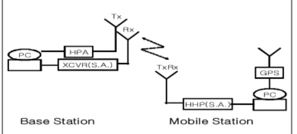
Fig. 4. Configuration of the Field Test Measurement System
2. Measurements for the RSSIs
The equipment parameters in figure 4 and link budget between the transmitter and receiver equipment are shown in table 1. The link budget makes it possible to obtain the path loss characteristics between the base station and mobile station in equation (10)[5].
Path Loss = P(Tx) - Tx. Antenna Cable Loss + Tx. Antenna Gain
- {P(Rx) - Rx. Antenna Gain
+ Rx. Antenna Cable Loss} (10) Radio dead spots and fading phenomenon make the path losses different even on the same distance between the transmitter and the receiver. The curvature of the terrain, obstacles due to the non-line of sight areas, buildings, and forests etc are the causes of the irregularities in the path loss.
Table 1. Link Budget of the measurement system
Base Station
Antenna Gain(dBd) Omni-direction 8 Direction(60) 12 Antenna Cable Loss(dB) 8 ~ 20 LNA Gain at the receiver(dB) 12
LNA NF at the receiver(dB) 2
Handset Antenna Gain(dBd) 3
Antenna Cable Los(dB) 3 ~ 6
The path losses according to the distance between transmitter and receiver are obtained in figure 5 from the measured RSSIs [7][8] with the environment parameters such as antenna gain and antenna cable losses etc.
0 5 10 15 20 25 30 35 40
100 110 120 130 140 150 160 170
Path Loss Measurement Results for Tx Ant. Height = 50m, Rx. Ant. Height = 3m and Isotropic Antenna
Distance, Km
Path Loss, dB
Fig. 5. The Path Loss Analyzed from the Field Test Measurement Data
3. The partial interval analysis to set-up the propagation model
After the formulas for the propagation models introduced in article II are normalized for the same measurement environment conditions, actually-measured data was drawn with the normalized formulas in figure 6[9][10].
The means and standard deviations for the difference between actually-measured data and the formulas are listed in table 2.
From the table, the average of the difference values between the measured data and Hata suburban model is -4.2 dB which is the minimum value, and the standard deviation of the difference values between the measured data and the direct wave and ground-reflected wave model or Egli model is 7.1 dB as the lowest value[11].
First, the entire distance is divided to 6 parts with 5 Km interval for analysis. And then, 6 representative models for 5 Km intervals which were selected among the conventional propagation models are shown in figure 7. The standard deviation between 6 partial interval-propagation models and the measured data is 5.8 dB, which is 1.3 dB lower than 7.1 dB, the standard deviation between the direct and ground-reflected model and the measured data.
0 5 10 15 20 25 30 35 40 80
90 100 110 120 130 140 150 160 170
180 Path Loss Models for Tx Ant. Height = 50m, Rx. Ant. Height = 3m and Isotropic Antenna
Distance, Km
Path Loss, dB
Free Space Plane Earth Egli HATA Urban
HATA SubUrban
HATA Open Measured Data
Free Space Plane Earth Egli HATA Urban HATA Sub-Urban HATA Open
Fig. 6. The path loss characteristics at the PNG in Russia Table 2. Comparisons of Means and standard deviations
Propagation models Mea
n Standard
Deviation Free Space Model 27.6 11.6 Direct-reflected Model 20.7 7.1
Egli Model -7.9 7.1
Hata Urban Model -14 8.1
Hata Suburban Model -4.2 8.1
Hata Rural Model 14.2 8.1
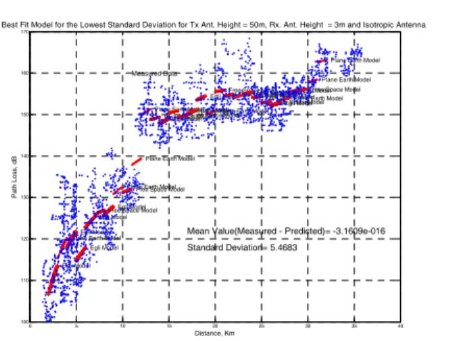
Next, the entire distance is divided to about 30 parts of 1 Km interval. 30 representative models for 1 Km intervals which were selected among the conventional propagation models are also shown in Figure 8. The standard deviation between 30 partial interval propagation models and the measured data is 5.4 dB, which is 0.4 dB lower than 5.8 dB, the standard deviation between 6 parts with 5 Km interval propagation model and the measured data.
0 5 10 15 20 25 30 35 40
100 110 120 130 140 150 160 170
Free Space Model Plane Earth Model
Free Space Model
Plane Earth ModelFree Space Model Plane Earth Model Best Fit Model for the Lowest Standard Deviation for Tx Ant. Height = 50m, Rx. Ant. Height = 3m and Isotropic Antenna
Distance, Km
Path Loss, dB
Mean Value(Measured - Predicted)= 3.4704e-015 Standard Deviation= 5.8761
Measured Data
Fig. 7. The path loss characteristics(Interval : 5 Km ) Table 3. Comparison of the Standard deviations(Intervals : 30Km, 5Km, 1Km)
Interval
Propa. Model Entire
Distance 5
Km 1 Km
Direct-Reflected Model 7.1
5.8 5.4
Egli Model 7.1
0 5 10 15 20 25 30 35 40
100 110 120 130 140 150 160 170
Egli Model Plane Earth ModelEgli Model
Egli Model Egli Model
Free Space Model Egli Model Plane Earth ModelFree Space Model
Plane Earth Model Plane Earth Model
Free Space Model Egli Model Free Space Model
Free Space Model Egli Model Egli Model
Plane Earth Model Free Space Model
Free Space Model Plane Earth ModelFree Space Model Free Space Model
Free Space Model Egli ModelPlane Earth Model Egli ModelFree Space Model
Plane Earth Model Plane Earth Model Best Fit Model for the Lowest Standard Deviation for Tx Ant. Height = 50m, Rx. Ant. Height = 3m and Isotropic Antenna
Distance, Km
Path Loss, dB
Mean Value(Measured - Predicted)= -3.1609e-016 Standard Deviation= 5.4683
Measured Data
Fig. 8. The path loss characteristics(Interval : 1 Km ) The standard deviations between the measured data and the entire distance, 5-Km, and 1-Km interval path loss models are summarized in table 3. The standard deviations for the 5-Km interval propagation model and the 1-Km interval propagation model are 5.8 dB, 5.4 dB respectively from table 3. As the result, the 5-Km model is 1.3 dB lower than the entire distance model.
And, The 1-Km model is 1.7 dB lower than the entire distance model.
In this paper, the propagation characteristics in the cellular band are measured at the PNG area in Russia, and then the path loss model could be analyzed from the data.
The best path loss model for the measured area, the PNG sites could be set up by the conventional propagation models.
By the partial interval analysis, the measured data at the PNG is used to find out the new-combined model from the conventional propagation models.
The entire measured data of 30 Km is divided to each 5-Km, or 1-Km interval, and the conventional propagation models were selected for each 5-Km or 1-Km interval propagation models. For each 5-Km or 1-Km interval, the means and standard deviations for the differences between the measured data and the conventional propagation models were obtained.
When a single conventional propagation model is applied to the measured data, the direct and ground-reflected propagation model is the closest to the measured data because the standard deviation between the measured data and the direct and ground-reflected propagation model is the smallest value of 7.1 dB.
The entire 30 Km distance is divided to 6 parts of 5 Km interval. And 6 models which are representative for each 5 Km
Kyung-tae Park (Member)
received the B.S. and M.S. degrees in electric and electronics engineering from KAIST in 1990 and 1992, respectively. He received the Ph.D degree in radio communication engineering from Korea Maritime University in 2011.
During 1992 ~ 1995, he was a research engineer at Samsung Electronics, Seoul, Korea. Since 1999, he joined the department of electronics and communications engineering at Masan University, where he is currently an associate professor.
His research interests include mobile communications, microwave devices, and linear power amplifiers.
Sung-hyuk Bae received the B.S. in electronics engineering from Dong-Kuk University, Korea in 1985. He received the M.S. in information technology engineering from Mok-Won University, Korea in 2009, and also completed the doctorial program in 2012. Since 1999, he joined the department of electronics and communications engineering at Masan University, where he is currently an associate professor.
His research interest is the electronic information security engineering.
interval are selected among the conventional propagation models.
The standard deviation between 6 partial models and the measured data is 5.8 dB. And the entire distance is divided to 30 parts of 1 Km interval. 30 models which are representative for each 1 Km interval are selected among the conventional propagation models. The standard deviation between 30 partial interval propagation models and the measured data is 5.4 dB.
By applying the partial interval propagation models to the cellular sites at the PNG in Russia, the standard deviation between the new-combined partial propagation model and the measured data is at least 1.7 dB improved.
Futhermore, by applying more conventional propagation models to the partial interval analysis method, the more accurate propagation model for the specific area is to be found out.
[1] Ki-Hong Song, "Development of Microcellular Radio Propagation Prediction Model in the 8 GHz Bands", Korea Institute of Electromagnetics and Engineering Science, Vol.17 No.12, pp. 1212-1223, Dec. 2006.
[2] William C. Y. Lee, "Mobile Cellular Telecommunications", McGraw-Hill Book Co., 1995.
[3] IEEE Vehicular Techology Society Committee on Radio Propagation, "Coverage Prediction for Moblie Radio System Operating in the 800/900 ㎒ Frequency Range", IEEE Transactions on Vehicular Techology, vol.37, No.1, pp. 3-72, Feb. 1988.
[4] Masaharu Hata, "Empirical Formula for Propagation Loss in Land Mobile Radio Services", IEEE Transactions on Vehicular Techology, vol.VT-29, No.3, pp. 317-325, Aug.
1980.
[5] Sang-Keun Lee, Hyo-Chang Bang, “CDMA Mobile Technology”, Sehwa, 2000.
[6] Kyung-Tae Park, Hyung-Rae Cho, “A Study on the Partial Path Loss Model By Using the Free Space and Hata Path Loss Model”, Korea Institute of Signal Processing and Systems, Vol.12 No.3, pp. 194-198, Aug.
2011.
[7] Myung-Sun Choi, Do-Yun Kim, Han-shin Jo, Cheul Mun, Jong-Gwan Yook, Han-Kyu Park, “Radio Propagation Characteristics in Subway Tunnel at 2.65 GHz”, Korea Institute of Electromagnetics and Engineering Science, Vol.16, No.5, pp. 541-548, 2005.
[8] Hironari Masui, Masanori Ishii, Kozo Sakawa, Hiroyuki Shimizu, Takehiro Kobayashi, and Masami Akaike,
"Microwave Path-Loss Characteristics in Urban and NLOS Environments", Vehicular Technology Conference,
VTC 2001 Spring, IEEE VTS 53rd, pp. 349-354, 2001.
[9] M. Yang, W. Shi, "Linear Least Square Method of Propagation Model Tuning for 3G Radio Network Planning", Fourth International Conference on Natural Computation ICNC, Jinan, pp. 150-154, 18-20 Oct. 2008.
[10] B. S. L. Castro, I. R. Gomes, F. C. J. Robeiro, and G. P.
S. Cavalcante, "COSTA231-Hata and SUI Models Performance Using a LMS Tuning Algorithm on 5.8 GHz in Amazon Region Cities", Antennas and Propagation, 2010 Proceedings of the Fourth European Conference, 2010.
[11] Popoulis, “Probability, Random Variables, and Stochastic Processes”, McGraw Hill Book Co., 1991.
[12] Mahdi Orooji and Bahma Abolhassani, "New Method for Estimation of Mobile Location Based on Signal Attenuation and Hata Model Signal Prediction", Proceedings of the 2005 IEEE Engineering in Medicine and Biology 27th Annual Conference, pp. 6025-6028, Sep.
2005.