ISSN 1225-7842 / eISSN 2287-402X http://dx.doi.org/10.7779/JKSNT.2016.36.2.93
Analysis of Time Domain Active Sensing Data from CX-100 Wind Turbine Blade Fatigue Tests for Damage Assessment
Mijin Choi*,****, Hwee Kwon Jung**, Stuart G. Taylor***, Kevin M. Farinholt***, Jung-Ryul Lee**** and Gyuhae Park**
Abstract This paper presents the results obtained using time-series-based methods for structural damage assessment.
The methods are applied to a wind turbine blade structure subjected to fatigue loads. A 9 m CX-100 (carbon experimental 100 kW) blade is harmonically excited at its first natural frequency to introduce a failure mode.
Consequently, a through-thickness fatigue crack is visually identified at 8.5 million cycles. The time domain data from the piezoelectric active-sensing techniques are measured during the fatigue loadings and used to detect incipient damage. The damage-sensitive features, such as the first four moments and a normality indicator, are extracted from the time domain data. Time series autoregressive models with exogenous inputs are also implemented. These features could efficiently detect a fatigue crack and are less sensitive to operational variations than the other methods.
Keywords: Structural Health Monitoring (SHM), Time Series Analysis, Piezoelectric Active Sensor, ARX Model
[Received: October 12, 2015, Revised: January 8, 2016 / March 9, 2016, Accepted: March 10, 2016] *Department of Aerospace Engineering & LANL-CBNU Engineering Institute, Chunbuk National University, Jeonju 54896, Korea,
**School of Mechanical Engineering, Chonnam National University, Gwangju 61186, Korea, ***The Engineering Institute, Los Alamos National Laboratory, Los Alamos, NM, 87544, USA, ****Department of Aerospace Engineering, KAIST, Daejeon 34141, Korea, Corresponding Author: [email protected]
2016, Korean Society for Nondestructive Testing
1. Introduction
Wind turbines are becoming a larger source of renewable energy in the world. The sizes of turbine blades, often made of composite materials, are increased to maximize the power output.
However, large composite structures are prone to in-service damage and manufacturing defects, which can lead to catastrophic failure under fatigue loads [1-12]. Blade damage is the most expensive type of damage to repair and can cause serious secondary damage to the overall wind turbine system due to rotating imbalance.
Therefore, it is imperative that a structural health monitoring (SHM) system be incorporated into the design of the wind turbines in order to monitor flaws to prevent a catastrophic failure.
SHM is defined as implementing a damage detection strategy for aerospace, civil and mech-
anical engineering infrastructure. SHM requires the application and the development of statistical models for discrimination between the damage sensitive features from the undamaged and damaged structures. A damage-sensitive feature is some quantity extracted from the measured system response data that indicates the presence of damage in a structure. Identifying features that can accurately distinguish a damaged structure from an undamaged one is the focus of most SHM technical literature.
The goal of this study is to assess time-
domain data measured for embedded piezo-
electric active-sensors as a way to nondestruc-
tively monitor the health of wind turbines. This
study uses the first four statistical moments and
a normality test to assess the condition of the
wind turbine blade under fatigue loads. The
underline assumption of this approach is that the
Fig. 1 CX-100 fatigue test set-up
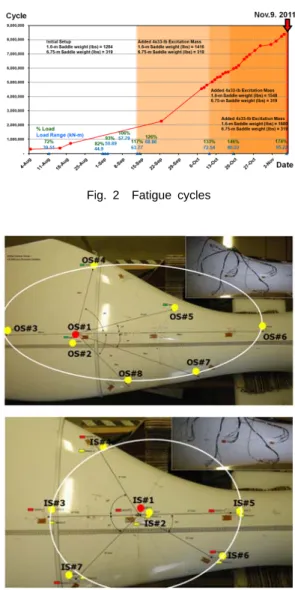
Fig. 2 Fatigue cycles
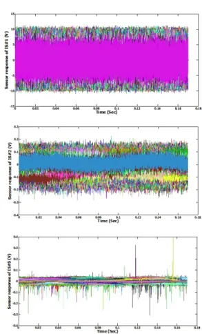
Fig. 3 Piezoelectric active sensor array (top: inner sensor array, bottom: outer sensor array)
high-frequency excitation of piezoelectric trans- ducer is sensitive enough to detect incipient crack in a structure and insensitive to operational vibrations. After then, time-series autoregressive models with exogenous inputs (ARX) are also implemented and a residual error between the measured and the predicted signals is used as a damage-sensitive feature. The results of these two approaches were compared that they reached the similar conclusion. The experimental setup and the analysis procedures are detailed in the next sections.
2. Experimental Setup
To develop a real-time SHM system for wind turbines, a full-scale fatigue test was performed in the period 08/11/2011 to 11/09/2011. The test set-up is shown in Fig. 1. The specimen is 100 kW blade, referred to as CX-100, which contains a full-length carbon spar cap infused with the rest of the blade as part of the normal glass blade fabrication process. This 9 m turbine blade was mounted to the 7 ton test stand and harmonically excited by its first natural frequency at 1.8 Hz to introduce failure modes [13]. The blade was initially excited at 25% of its design load, and then the load was steadily increased until the blade failed as shown in Fig. 2. To induce the fatigue loading, a UREX (universal resonant excitation) hydraulic actuator (load saddle) was installed at the 1.6 m spanwise station with a single ballast saddle located at the 6.75 m from the root, respectively, and extra masses were added on the first load saddle at 1.6 m, leading to increase of mass from 1,284 lbs initially to 1,416, 1,548, 1,680 lbs respectively. For more details on the experi- mental set-up, see References [13,14].
In piezoelectric sensing systems, two different
sensor arrays, designated in this paper as inner
and outer, were implemented, as shown in
Fig. 3. All transducers utilized in this study
Fig. 5 Time-series raw data of inner sensor array (IS#1, IS#2, IS#5)
Fig. 4 A through-thickness fatigue crack on CX-100
were APC International D-0.500-0.020-851 PZT transducers, fabricated using the APC’s 851 material. The transducers were 12 mm diameter and 0.5 mm thickness. The inner sensor array observed a 0.75 m region centered 1 m from the blade’s root, while the outer array observed 2 m elliptical region centered 1.5 m from the root.
A patch in the middle of the circular array was used as an actuator, providing band-limited white noise excitation from 500 Hz to 40 kHz over a voltage range of
±10V, and other neighbor sensors measured the corresponding responses had 16,384 points sampled at 96 kHz, for a duration of 170.67 ms. The measurements were made 565 times for the inner array and 534 times for the outer array from 08/11/2011 to 11/09/2011, respectively, while the blade was under continuous fatigue loads.
A through-thickness fatigue crack surfaced on the blade transitional root area as shown in Fig. 4. This damage was estimated to be initiated nearby IS#5, propagated to IS#6 over time and finally visually identified on 11/09/2011 at fatigue load cycle approximately 8.5 million cycles.
3. Time-Series Analysis 3.1. Time-Series Raw Data
To assess the quality of the measured signals, the raw time series of the inner array (IS1, IS2, and IS5) are overlaid and plotted with the data
measured from 08/11/2011 to 11/09/2011 in Fig.
5. Each color represents a measured raw data for each date during the fatigue tests. The raw time domain data of IS#1 represents excitation signals.
The sensor response of the IS#2 shows responses close to the white noises as the input signals. Some ‘spiky’ signals were observed from IS#5, which sensors were placed relatively close to the identified damage. It is speculated that these spiky responses are generated by acoustic emission activities, when damage is initiated on the thick root and is excited by the applied load.
3.2. First Four Statistical Moments
To identify the presence of damage, the first
-2 -1.5 -1 -0.5 0 0.5 1 1.5 2 0.001
0.003 0.01 0.02 0.05 0.10 0.25 0.50 0.75 0.90 0.95 0.980.99 0.997 0.999
Data
Probability
Normal Probability Plot of IS5
SEP 23rd OCT 19th NOV 8th
Fig. 8 Normal probability plots of IS#5
-2 -1.5 -1 -0.5 0 0.5 1 1.5 2
0.001 0.003 0.01 0.02 0.05 0.10 0.25 0.50 0.75 0.90 0.95 0.98 0.99 0.997 0.999
Data
Probability
Normal Probability Plot of IS6
SEP 23rd OCT 19th NOV 9th
Fig. 9 Normal probability plots of IS#6
0 100 200 300 400 500
-8 -6 -4 -2 0 2 4 6
Number of tests
Skewness
IS#2 IS#3 IS#4 IS#5 IS#6 IS#7
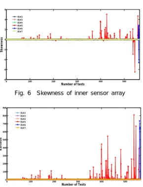
Fig. 6 Skewness of inner sensor array
0 100 200 300 400 500
0 100 200 300 400 500 600 700 800 900
Number of Tests
Kurtosis
IS#2 IS#3 IS#4 IS#5 IS#6 IS#7
Fig. 7 Kurtosis of inner sensor array
four statistical moments (mean, standard devi- ation, skewness, and kurtosis) were computed from the measured data. As can be seen in Figs.
6 and 7, significant deviation of skewness and kurtosis were observed in the measurement taken from of IS#5 (red line) and IS#6 (blue line), which are located quite near the identified crack.
Both skewness and kurtosis of IS#5 signals started to be diverged from zero continually after 10/19/2011 and it reached maximum value on 11/08/2011. In the signals from IS#6, each skewness and kurtosis also increased dramatically prior to the failure, when the crack surfaced.
The changes associated with skewness and kurtosis should be understood, as the changes with the feature distribution, which may be caused by nonlinearity associated with the damage. The authors believe that these results indicate that the damage was initiated and detected by tracking these features as early as 21 days prior to the visual crack. It should be noted, however, that The mean and standard deviation did not show any meaningful changes
with the presence of damage. In addition, the skewness and kurtosis of the outer sensors did not give any insight about the presence of damage. In other words, sensors should be installed close to the damage location in order to efficiently detect the presence of damage.
3.3. Normality Test
The normal probability plot is a graphical method for normality test. It could be considered to be linear when the data come from a normal distribution. If the data are related to another probability distribution, which could be caused by structural damage, a curvature will be introduced as shown in the plot. Fig. 8 shows the normal probability plots for three dates, Sep.
23rd, Oct. 19th, and Nov. 8th, for the IS#5.
For the data measured on 09/23/2011 in the
initial stage of the fatigue test, the distribution
of IS#5 signal was Gaussian and it could be
considered the wind turbine structure behave
linearly. On 10/19/2011 when the skewness and
kurtosis of IS#5 were started to show huge deviations as shown in the previous section, there was a curvature in the tail of the distribution of IS#5.
Fig. 9 shows the normal probability plots for three dates, Sep. 23rd, Oct. 19th, and Nov. 9th, for the IS#6. Both the data measured on 09/23/2011 and 10/19/2011, the distribution of IS#6 signal was Gaussian and it could be considered the structural damage was not propagate to the location IS#6 placed. However, on 11/09/2011 when the skewness and kurtosis of IS#6 present dramatically changes as shown in Fig. 6 and Fig. 7, there was a curvature in the tail of the IS#6 signal distribution as same as IS#5’s. This could be concluded that unusual sources of variability exist nearby IS#5 and then propagate to the location IS#6 installed during the fatigue test. These results strongly support the conclusion of the previous section.
One conclusion could be drawn that, without using any advanced signal processing techniques to extract a damage sensitive feature, the basic four statistical moments could be efficiently used to detect and locate structural damage. This is mainly because the frequency range used to interrogate structural components is high and sensitive enough to detect and locate structural damage, and insensitive to operational vibration, i.e. fatigue loadings.
3.4. Autoregressive Model with Exogenous Inputs
Finally, time series predictive models, such as an autoregressive model with exogenous inputs (ARX), are used for damage assessment.
In time series ARX model analysis,
which is measured signal at discrete time index
can be defined with its finite past series and input history as;
1
1 0
( )
p q
j i j i k i
j k
x t φ s
− −β v
−e
= =
= ∑ + ∑ +
where
is called AR coefficients,
and
define the orders in the ARX model and
is the residual error at the signal value
after fitting the ARX(p,q) model to the
and
pair [15].
The appropriate order of the ARX model is initially unknown. A high-order model may perfectly predict measured data, but will not generalize to other data sets. On the other hand, a low-order model will not necessarily fit the underlying physical system response. Therefore, it is important to determine the optimal model order to the ARX model development. In order to computing the optimal model order, the root mean squared error (RMSE) technique was implemented in this study. In the ARX model, the RMSE is a measure of the differences between the values estimated by model and the values actually measured. The results suggest that an AR model of order p=q=80 would fit the time response reasonably well because the RMSE flats around p=q=80.
Fig. 10 shows overlaid plots of the measured and estimated time histories at IS#6 for 08/23/2011 using ARX (80, 80) model for representing how well the model fit the data.
From a qualitative point of view windowed time histories with 50 points, shown in Fig. 9, illustrate that ARX (80, 80) model developed from the baseline condition appear to predict the data well.
In this study, damage features were extracted
using residual errors between measured data and
ARX model predicted data. Fig. 11 shows
probability density functions of the residual
errors which had been estimated with the kernel
density procedure. As shown in Fig. 11, the
residual error of IS#5 and IS#6 on 09/23/2011
showed symmetric distribution and smaller
standard deviation. But they kept changing into
asymmetric distribution during the fatigue test
and had the largest standard deviation on
11/08/2011. The reason of this variation is that
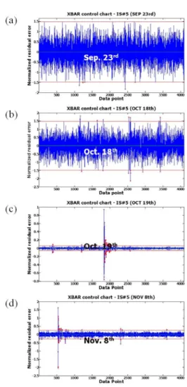
Fig. 12 Control charts of measured time histories of IS#5: (a) 09/23/2011, (b) 10/18/2011, (c) 10/19/2011, (d) 11/08/2011
Fig. 10 Comparison of the measured data and estimated time histories using ARX (80,80) model fit to Aug. 23rd data from IS#6
-1 -0.8 -0.6 -0.4 -0.2 0 0.2 0.4 0.6 0.8 1
0 2 4 6 8 10 12 14
Residual error
SEP 23rd OCT 18th OCT 19th NOV 8th NOV 9th
Fig. 11 Probability density functions of residual errors over time
system is changed to a new state (damaged condition) and the ARX models, which is constructed under the undamaged condition, is not able to predict the damaged response.
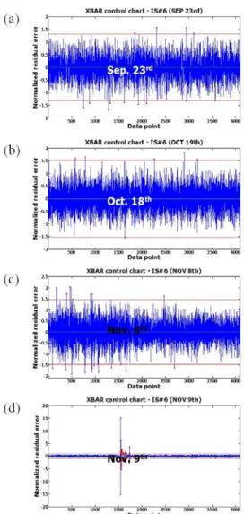
Another approach of damage features extrac- tion is an X-bar control chart analysis. The X-bar control charts are used to identify when data points fall outside the control limits and these points are called ‘outliers’. Physically, outliers indicate that the structure has an unusual source of variability that deviates from the baseline
condition. Fig. 12 illustrates X-bar control charts of residual errors between measured data from IS#5 and its ARX model on 09/23/2011 (intial stage of fatigue test), 10/19/2011 (when skewness and kurtosis of IS#5’s signal started to be changed), and 11/08/2011 (when skewness and kurtosis of IS#5’s signal were the largest value), respectively.
As shown in Fig. 12, the number of outliers
beyond the control limits was small on
09/23/2011 and 10/18/2011 but it was suddenly
increased after 10/19/2011 and outliers kept
increasing until 11/08/2011. Fig. 13 plots an
Fig. 13 Control charts of measured time histories of IS#6: (a) 09/23/2011, (b) 10/18/2011, (c) 11/08/2011, (d) 11/09/2011