http://dx.doi.org/10.4134/JKMS.2012.49.5.927
A REGULARIZED CORRECTION METHOD FOR ELLIPTIC PROBLEMS WITH A SINGULAR FORCE
Hyea Hyun Kim
Abstract. An approximation of singular source terms in elliptic prob- lems is developed and analyzed. Under certain assumptions on the curve where the singular source is defined, the second order convergence in the maximum norm can be proved. Numerical results present its better per- formance compared to previously developed regularization techniques.
1. Introduction
Singular force terms in differential equations model discontinuities of solu- tions which arise in interaction of fluid and an elastic structure immersed in it.
Immersed boundary methods developed by Peskin [8, 9] provide a sound math- ematical model for such interactions. Numerical solutions of the suggested mathematical model require accurate approximation of singular force terms, such as Dirac delta distribution. In the work, regularized Dirac delta distribu- tion is used and this results in less satisfactory convergence for two- and three- dimensional problems.
Another approach treating such problems is to find correction terms in fi- nite difference operators and to make the truncation error within a required accuracy. This can be done by incorporating the discontinuities of solutions and their derivatives across the elastic structure and the geometric properties of the structure, such as curvature and tangent. This kind of approach has been studied and developed by Mayo [6, 7], and by Leveque and Li [5]. For these methods, second order convergence has been achieved and mathematical analysis has also been provided. In the both methods, it is quite complicated to approximate geometric properties of the structure as well as to find correction terms.
Received September 10, 2010.
2010 Mathematics Subject Classification. 65N30, 65N55, 76D07.
Key words and phrases. Dirac delta function, second order methods, immersed boundary.
This research was supported by Basic Science Research Program through the National Research Foundation of Korea(NRF) funded by the Ministry of Education, Science and Technology(2009-0065373).
⃝2012 The Korean Mathematical Societyc 927
Regularization methods approximate the singular source by employing func- tions, which satisfy certain physical properties, such as momentum condition.
In practice, regularization methods are widely used due to their much simpler implementation of the singular force terms. However, in two or three dimen- sional problems they give approximated solutions with only first order accuracy near the interface, see Tornberg and Engquist [10, 11].
In this work, we develop a regularization method with a better accuracy for approximating the singular source term. We consider elliptic problems in a two dimensional domain with the source term given by Dirac delta distribution on a closed curve inside the domain. In our approach, we approximate the geometric property of the curve by introducing polygons and then find an approximation to the singular force term by using the integral of the fundamental solution over the polygons.
Under certain assumptions on the curve, we can prove the second order convergence of our approximation. The geometric properties of the curve is implicit in the polygons. This fact makes our approach as simple as the exist- ing regularization methods and also provides as good accuracy as the existing correction methods. In numerical results, we observe less satisfactory conver- gence of solutions for the models with the interface which does not satisfy the assumptions. However, its convergence is observed to be better than the previously developed regularization methods.
In Section 2, we introduce a model problem and in Section 3 we describe the method for approximating the singular force terms by using polygons. We provide analysis for accuracy of our approach in Section 4 and we present numerical results in Section 5. Throughout this paper, C denotes a generic positive constant which does not depend on the discretization parameter h.
2. Model problem and discretization We consider a model problem:
Find u ∈ Ω such that
△u(x) = δ(γ, x) ∀x ∈ Ω, u(x) = g(x) ∀x ∈ ∂Ω, (2.1)
where Ω is a domain in R
2and γ is a smooth closed curve inside Ω, which is a codimension-one subset of Ω. Here δ(γ, x) is a Dirac delta distribution which is defined by
∫
Ω
δ(γ, x)v(x) dx =
∫
γ
v(x(s)) dx(s)
for any function v(x) in H
s(Ω) with s > 1/2. Here, H
s(Ω) is the Sobolev space of functions such that their weak derivatives up to s are square integrable.
We assume that Ω is a rectangular domain in R
2. We introduce uniform grid
points in the domain Ω and denote the set of grid points by Ω
h. The model
problem is then discretized on the given grid points,
△
hU (x
i) = F (x
i), ∀x
i∈ Ω
h∩ Ω, U (x
i) = g(x
i), ∀x
i∈ Ω
h∩ ∂Ω, (2.2)
where U (x
i) denotes an approximate solution at the grid point x
iand △
hU (x
i) is a discrete Laplacian,
(2.3) △
hU (x) = U (x
L) + U (x
R) + U (x
D) + U (x
U) − 4U(x)
h
2.
Here x
L, x
R, x
D, and x
Uare grid points which are located at one grid width left, right, down, and up from the grid point x. In the following section, we will look for a good approximation of F (x
i) to the singular source term, which produces a discrete solution U of u such that
max
xi∈Ωh
∥U(x
i) − u(x
i) ∥ ≤ Ch
2under certain assumptions on γ.
3. Approximation of the singular source term
We will propose an efficient way to approximate the singular force. We consider
(3.1) v(x) =
∫
γ
Γ(x, y(s)) dy(s), where Γ(x, y) is the fundamental solution,
Γ(x, y) = 1
2π log |x − y|.
The function v(x) then satisfies that ∆v(x) = δ(γ, x). If v(x) = g(x) on ∂Ω, v(x) is the exact solution of (2.1). This is not the case in general.
With the help of v(x), we will find a good approximation F of δ(γ, x), which appears in the discrete form (2.2). We decompose the solution u(x) into two parts,
u(x) = v(x) + w(x).
We call v(x) the singular part and w(x) the regular part. Then w(x) satisfies that
∆w(x) = 0, ∀x ∈ Ω,
w(x) = u(x) − v(x), ∀x ∈ ∂Ω.
(3.2)
For the smooth function w(x), we can approximate ∆w at the grid point x with the second order accuracy using the Taylor series expansion, i.e.,
(3.3) ∆w(x) = w(x
L) + z(x
R) + w(x
D) + w(x
U) − 4w(x)
h
2+ O(h
2).
We introduce the notation A for the matrix of the discrete Laplacian Au(x) = u(x
L) + u(x
R) + u(x
D) + u(x
U) − 4u(x)
h
2.
Lemma 3.1. For a point x = (x, y) with its four neighbors on the same side of γ, we have
Av(x) = h
24!
∑
z∈N(x)
( ∂
4∂x
4∫
γ
log |x − y(s)| dy(s) )
x=z
,
where N (x) is a set with four points near x.
Proof. We consider (3.4)
Av(x, y)h
2=
∑
2 k=1( v(x + ( −1)
kh, y) − v(x, y) ) +
∑
2 k=1( v(x, y + ( −1)
kh) − v(x, y) ) . By the Taylor series expansion, we obtain
v(x ± h, y) − v(x, y) = v
x(x, y)( ±h) + 1
2! v
xx(x, y)( ±h)
2+ 1
3! v
xxx(x, y)( ±h)
3+ 1
4! v
xxxx(ξ
x±, y)( ±h)
4, v(x, y ± h) − v(x, y) = v
y(x, y)( ±h) + 1
2! v
yy(x, y)( ±h)
2+ 1
3! v
yyy(x, y)( ±h)
3+ 1
4! v
yyyy(x, ξ
y±)( ±h)
4, where ξ
x±and ξ
±yare points between x ± h and x, and between y ± h and y, respectively.
Since v
xx(x, y) + v
yy(x, y) = 0, Av(x, y) = 1
4!
∑
z=ξ+x, ξ−x
v
xxxx(z, y)h
2+ 1 4!
∑
z=ξy+, ξ−y
v
yyyy(x, z)h
2.
By selecting N (x) = {(ξ
x+, y), (ξ
x−, y), (x, ξ
y+), (x, ξ
y−) } and using v
xxxx= v
yyyy,
we complete the proof. □
For the curve γ, we assume that γ ∈ C
4+αwith 0 < α < 1. Let Ω
+(γ) and Ω
−(γ) denote the subregions of Ω which are outside and inside γ, respectively.
We use v
±to denote the restriction of v to Ω
±(γ), respectively. The function v in (3.1) then satisfies
△v = 0 in Ω
±(γ) with the interface conditions on γ
v
+− v
−= 0, ∂v
+∂n − ∂v
−∂n = 1.
Here
∂v∂nis the normal derivative of v on γ.
We apply Lemma 2.4 of Beale and Layton [1] to the above model problem to obtain the following regularity result for v:
Lemma 3.2. Suppose γ ∈ C
4+αfor some 0 < α < 1. Then v
±∈ C
4+α(Ω
±(γ)).
Lemma 3.3. Let γ ∈ C
4+αbe a closed curve inside Ω with 0 < α < 1 and let dist(x, γ) be the distance from a point x to the curve γ. For a point x with dist(x, γ) > h, we obtain
Av(x) ≤ Ch
2. Proof. From Lemma 3.1, we obtain
Av(x) = h
24!
∑
z∈N(x)
∂
4v
∂x
4(z),
where N (x) is the set with four points near x which are within distance h from x. Since dist(x, γ) > h, the four points in N (x) are all inside γ or all outside γ. By Lemma 3.2, we obtain
Av(x) ≤ Ch
2. Here the constant C depends on
∂
4v
∂x
4(x)
L∞(Ω+(γ))
and ∂
4v
∂x
4(x)
L∞(Ω−(γ))
,
where ∥v∥
L∞(Ω)denotes the maximum norm of the function v in the domain
Ω. □
Among the uniform grid points, we denote the node points which are located within one grid width from the interface γ by x
irrand denote the other nodes by x
reg. At the grid points x
irrnear the interface γ, i.e., dist(x
irr, γ) ≤ h, we consider
Au(x
irr) = Aw(x
irr) + Av(x
irr).
Since w is smooth in Ω, see (3.2) and (3.3), we obtain (3.5) Au(x
irr) = Av(x
irr) + O(h
2).
In other words, we obtained a second order approximation of Au(x
irr) using Av(x
irr), which can be computed by using the values of v(x) at the point x near x
irr. The values of v(x) can be obtained from the Green’s formula (3.1).
At the other grid points x
reg, we apply Lemma 3.3 to Av to obtain (3.6) Au(x
reg) = A(v + w)(x
reg) = Av(x
reg) + O(h
2) = O(h
2).
We now obtain an approximation of the singular force F (x), F (x
irr) = Av(x
irr), F (x
reg) = 0, which satisfies that
(3.7) Au(x) − F (x) = O(h
2)
for any grid points x, see (3.5) and (3.6).
Theorem 3.4. Let F be given to satisfy (3.7). Then the solution U of AU = F
with U (x) = u(x) at the grid points x on ∂Ω, satisfies that
∥U − u∥
∞≤ Ch
2.
Proof. We note that the matrix of the discrete Laplacian satisfies
(3.8) c ≤ −A ≤ C 1
h
2, which is equivalent to
(3.9) C
−1h
2≤ −A
−1≤ c
−1.
Since F is chosen in such a way that
(3.10) F = Au + O(h
2),
and both u and U have the same boundary condition on ∂Ω, A(u − U) = Au − AU = Au − F = O(h
2).
Using (3.9), we finally obtain
∥u − U∥
∞≤ ∥A
−1∥
∞O(h
2) ≤ Ch
2,
where C denotes a generic positive constant independent of the grid size. □ 4. Approximation by polygons
In practice, we need to compute Av(x) at the grid points x near γ and the computation of Av(x) requires to evaluate v at the grid point x and at its four neighboring points. For a given curve γ, it is not easy to compute the exact value of
v(x) =
∫
γ
Γ(x, y) dy(s).
We now propose an efficient way to compute an approximation v
h(x) of v(x) and will use v
h(x) when we compute the force F . We will propose a v
h(x) which does not deteriorate the second order convergence.
To approximate v(x), we consider a polygon γ
hγwith its vertices on γ and with its side length comparable to h
γ. Let {a
i}
ni=0−1be the vertices of γ
hγand let l
ibe the line connecting a
i−1and a
i, and γ
iis the part of γ with the two end points a
i−1and a
i.
Under certain assumptions on γ, we will show that v
hsatisfies that
∥v
h(x) − v(x)∥ ≤ Ch
2.
Assumption 4.1. We divide the curve γ into {γ
i}
i, with the length of each γ
icomparable to h
γ, i.e.,
γ = ∪
i
γ
i.
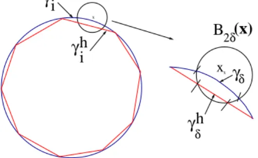
x
x
B
2δγ h
δ
γ i γ i
h
γ
δ(x) x
Figure 1. B
2δ(x), γ
i, l
i(= γ
ih) : γ
δand l
δ(= γ
δh) are part of γ
iand l
iwhich are within 2δ from the point x.
We parameterize each curve γ
ion the interval [0, h
γ] so that γ
i(s) = (x
0+ s, y
0+ g
i(s)) for s ∈ [0, h
γ] with g
i(0) = 0 and (x
0, y
0) to be the starting point of γ
i. For a sufficiently small h
γ, g
i(s) satisfies that
|g
i(s) | ≤ Ch
2γand |g
′i(s) | ≤ Ch
γ.
Lemma 4.2. Let γ be partitioned by {γ
i}
i, which satisfies Assumption 4.1 and h
γ≤ Ch
2. For a grid point x, we then have
∑
i
∫
γi
log |x − y(s)|dy(s) = ∑
i
∫
li
log |x − y(s)|dy(s) + O(h
2) for a sufficiently small h > 0. Here l
iis the straight line segment that connects the two end points of γ
i, h
γis the size of γ
i, and h is the grid size provided for Ω.
Proof. Let d
ibe the distance from a grid point x to γ
i, d
i= dist(x, γ
i),
where dist(x, A) denotes the distance from x to the set A. We consider E
i=
∫
γi
log |x − y(s)|dy(s) −
∫
li
log |x − y(s)|dy(s).
For γ
iwith d
i≤ h we will show that
∑
i,di≤h
|E
i| ≤ Ch
2,
and for the other case of γ
iwith d
i> h we will show that
∑
i,di>h
|E
i| ≤ Ch
2.
We choose δ = h
5/2and let B
δ(x) be the ball centered at x with the radius δ. Let
A
k= B
12k−1δ
(x) \ B
12kδ
(x) for all nonnegative integer k. Then
B
2δ(x) = ∪
k≥0
A
k. We introduce
γ
δ= γ
i∩ B
2δ(x) and l
δ= l
i∩ B
2δ(x), and then we have
γ
δ= ∪
k≥0
γ
δ,kand l
δ= ∪
k≥0
l
δ,k, where
γ
δ,k= γ
δ∩ A
kand l
δ,k= l
δ∩ A
k. In Figure 1, examples of such γ
i, l
i, and B
2δ(x) are presented.
Let γ
R= γ
i\ γ
δand l
R= l
i\ l
δ. For d
i≤ h, we consider E
i=
∫
γi
log |x − y(s)| dy(s) −
∫
li
log |x − y(s)| dy(s)
=
∫
γR
log |x − y(s)| dy(s) −
∫
lR
log |x − y(s)| dy(s) +
∫
γδ
log |x − y(s)| dy(s) −
∫
lδ
log |x − y(s)| dy(s).
We obtain
∫
γδ,k
log |x − y(s)| dy(s) ≤ C
−log( 1 2
kδ)
1
2
kδ = C(k log 2 − log δ) 1 2
kδ.
This bound gives that
∫
γδ
log |x − y(s)| dy(s) ≤ C
δ log 2 ∑
k≥0
k
2
k− δ log δ ∑
k≥0
1 2
k
≤ C(δ + δ
4/5δ
1/5( − log δ))
≤ Cδ
4/5≤ Ch
2. (4.1)
Here we have used that δ
1/5( − log δ) goes to zero as δ goes to zero and δ = h
5/2. Similarly, we can prove that
(4.2)
∫
lδ
log |x − y(s)| dy(s) ≤ Ch
2.
Without loss of generality, we may assume that γ
Ris parameterized by l
R,
γ
R= (x
0+ s, y
0+ g(s)), s ∈ l
R,
where (x
0, y
0) is the starting point of the γ
i. We then have
∫
γR
log |x − z(s)| dz(s) −
∫
lR
log |x − z(s)| dz(s) (4.3)
≤
∫
lR
log |(x, y) − (x
0+ s, y
0+ g(s)) | √
1 + (g
′(s))
2ds
−
∫
lR
log |(x, y) − (x
0+ s, y
0) | ds
≤
∫
lR
(log |(x − x
0− s, y − y
0− g(s))| − log |(x − x
0− s, y − y
0) |)
× √
1 + (g
′(s))
2ds +
∫
lR
log |(x − x
0− s, y − y
0) |( √
1 + (g
′(s))
2− 1) ds
≤ C (∫
lR
|y − y
0− ξ(s)|
(x − x
0− s)
2+ (y − y
0− ξ(s))
2|g(s)| ds +
∫
lR
log |(x − x
0− s, y − y
0) |(g
′(s))
2ds )
,
where ξ(s) is between zero and g(s). Here we have used that 1 ≤ √
1 + (g
′(s))
2≤ C. Since dist((x, y), γ
R) > 2δ, |ξ(s)| ≤ h
2γ≤ Ch
4, and δ = h
5/2, (x − x
0− s)
2+ (y − y
0− ξ(s))
2> δ
2, |(x − x
0− s, y − y
0) | > δ.
From the above bound, Assumption 4.1 and (4.3), we obtain
∫
γR
log |x − z(s)| dz(s) −
∫
lR
log |x − z(s)| dz(s)
≤ C (∫
lR
1
δ h
2γds +
∫
lR
| log(δ)|h
2γds )
≤ Ch
3γ1 δ . (4.4)
We note that there are
hhγ
number of such γ
iwith d
i< h and among them there is at most one such γ
iwhich intersect B
2δ(x) since δ = h
5/2< h
γ. Combining (4.1), (4.2), and (4.4), we obtain
∑
i,di≤h
∫
γi
log |x − y(s)|dy(s) −
∫
li
log |x − y(s)|dy(s)
≤ C
h
2+ ∑
i,di≤h
h
3γ1 δ
≤ C (
h
2+ h
3γ1 h
5/2h h
γ)
≤ Ch
2.
For the case (k + 1)h > d
i> kh with k ≥ 1, we have that
(x − x
0− s)
2+ (y − y
0− ξ(s))
2> (kh/2)
2, |(x − x
0− s, y − y
0) | > kh/2.
In a similar way to (4.4), we can prove that
|E
i| = ∫
γi
log |x − z(s)| dz(s) −
∫
li
log |x − z(s)| dz(s)
≤ C (∫
li
1
kh h
2γds +
∫
li
| log kh|h
2γds )
≤ Ch
3γ1 kh . Let 0 < ϵ < 1 be given. Since there are
hhγ
number of such E
i’s for each k, we obtain
∑
i,di>h
|E
i| ≤ C
∑
1/h k=1h
3γ1 kh
h h
γ≤ C
∫
1/h 11 x dxh
2γ≤ C| log h|h
2γ≤ Ch
2γh
−ϵh
ϵ| log h|
≤ Ch
4−ϵ≤ Ch
2.
Here we used that h
ϵ| log h| is bounded above by a constant for sufficiently
small h > 0. □
Remark 4.3. In the above, the error on the part of γ of which distance is larger than h from the point x is given by
∑
i,di>h
|E
i| < Ch
2γh
−ϵ.
Using this bound, by selecting larger h
γ= O(h) for a given point x with dist(x, γ) > h we can obtain
∥v(x) − v
h(x) ∥ ≤ Ch
2−ϵ,
which gives the error bound slightly less than the second order. In the numerical tests, with the choice of h
γ= h, the errors are observed regarding to the grid size h. Their behavior follows the second order, O(h
2) as h gets smaller. With the choice of h
γ= h
2, we observe O(h
4)-errors, which are consistent with our theory for the point x with dist(γ, x) > h.
Instead of v(x), we will use v
h(x) to compute F . By integrating the fun- damental solution on each line segment l
i, we can compute the exact value of v
h(x) by the formula
v
h(x) = 1 2π
∑
n i=1(U
i(x − a
i) − U
i(x − a
i−1)) , where a
n= a
0. Here
U
i(x) = x · t
i(1 − log |x|) − x · n
iarctan ( x · t
ix · n
i) ,
and t
iand n
iare unit tangent and unit normal to l
i, which is the straight line
segment connecting the two points a
i−1and a
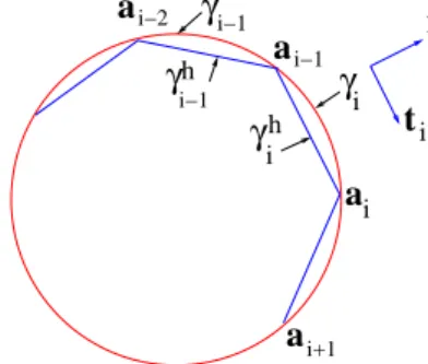
i, see Figure 2.
γ
i ha
a t
in
ia
a γ
iγ
i−1 hγ
i−1i+1 i i−1 i−2
Figure 2. γ
iand l
i(= γ
hi) : γ
ihis the straight line connecting the two points (a
i−1, a
i), and t
iand n
iare unit tangent and unit normal to γ
ih, respectively.
We compute an approximation of the singular force by using v
h(x) and obtain the following convergence result:
(4.5) ∥v
h(x) − v(x)∥ ≤ Ch
2.
Lemma 4.4. Let F
1= Av and F
2= Av
hwith ∥v − v
h∥
∞≤ Ch
2. Let U
1and U
2be the solutions of
AU
1= F
1, AU
2= F
2with U
1= U
2= u at the grid points on ∂Ω. If U
1satisfies ∥U
1− u∥
∞≤ Ch
2, then the same error bound holds for U
2, ∥U
2− u∥
∞≤ Ch
2.
Proof. Since U
1and U
2are solutions of
AU
1= F
1and AU
2= F
2,
with F
1= Av and F
2= Av
hand with the same boundary condition, U
1= U
2= u on ∂Ω, we obtain that
(4.6) U
1(I) − U
2(I) = A
−1IIA
II(v(I) − v
h(I)) − A
−1IIA
IB(v(B) − v
h(B)), where v(I) and v(B) stand for the vector of values of v(x) at the grid points in the interior of Ω and on the boundary of Ω, respectively. Similarly, the subscripts I and B in matrices denote that the columns and rows of the matrices correspond to the interior grid points and the grid points on the boundary of Ω, respectively. From
∥v − v
h∥
∞≤ Ch
2,
(4.6), and the discrete maximum principle, we obtain that
∥U
1(I) − U
2(I) ∥
∞≤ Ch
2.
If U
1satisfies that ∥U
1− u∥
∞≤ Ch
2, then the same bound holds for U
2,
∥U
2− u∥
∞≤ Ch
2. □
We note that v(x) satisfies that
Av(x) = O(h
2) for all x such that dist(x, γ) > h.
We will prove a similar bound for v
h(x). We then approximate Av
h(x) by zero at the grid points x located in a certain distance away from γ where Av
h(x) is negligible and we compute Av
h(x) at only the grid points near γ.
For a given 0 < ϵ < 1, let
d
min= max {3h, h
(4−ϵ)/4}.
In the following lemma, we will show that at a grid point x of which distance from γ
h= ∪
ni=1
l
iis larger than d
min,
|Av
h(x) | ≤ Ch
2.
Therefore we only need to compute Av
h(x) at the grid points which are within the distance d
minfrom γ
hand at the other grid points we can approximate Av
h(x) by zero to omit the computation of Av
h(x). The resulting force F then produces a second order approximation to u.
Lemma 4.5. Let 0 < ϵ < 1 be given and h
γ= O(h
2). At a grid point x
0whose distance from γ is d(x
0) which is larger than d
min,
d
min= max {3h, h
(4−ϵ)/4}, we obtain
(Av
h)(x
0) = O(h
2).
Proof. We recall the proof in Lemma 3.1. Since v
h(x) is smooth except γ
hγ, as in the proof of Lemma 3.1 for x
0with d(x
0) > d
minwe obtain
(4.7) (Av
h)(x
0) = 1 4!
∑
z=ξ+x, ξx−
(v
h)
xxxx(z, y
0)h
2+ 1 4!
∑
z=ξ+y, ξ−y
(v
h)
yyyy(x
0, z)h
2,
where ξ
x±is between x
0and x
0±h, and ξ
y±is between y
0and y
0±h, respectively.
Here we note that x
0= (x
0, y
0). We will prove that
(4.8) (v
h)
xxxx(ξ
x±, y
0) ≤ C and (v
h)
yyyy(x
0, ξ
±y) ≤ C.
The assertion of the lemma will then follow.
Let w(x) = v(x) −v
h(x) and B
r(x
0) be a ball centered at x
0with the radius r. Let d = d(x
0). Since dist(x, γ) > (1/3)d > h for all x ∈ B
(2/3)d(x
0), we obtain
(4.9) |w(x)| ≤ Ch
4−ϵ, ∀x ∈ B
(2/3)d(x
0),
see Remark 4.3. Since w(x) is harmonic in B
(2/3)d(x
0), it satisfies that (4.10)
∂
4w
∂x
4(x)
≤ C 1
(d/3)
4max
x∈B(2/3)d(x0)
|w(x)|, ∀x ∈ B
(1/3)d(x
0),
see derivative estimates for harmonic functions in [3, Theorem 2.10]. From (4.9) and (4.10),
∂
4v
h∂x
4(x) ≤ C (
∂
4v
∂x
4(x) + h
4−ϵd
4)
, ∀x ∈ B
(1/3)d(x
0).
By using Lemma 3.2, (ξ
x±, y
0) ∈ B
(1/3)d(x
0), (x
0, ξ
±y) ∈ B
(1/3)d(x
0), and d >
h
(4−ϵ)/4, we prove the bounds in (4.8). □
Remark 4.6. The proof is valid for a more general choice of d
minsuch that d
min= max {ch, h
(4−ϵ)/4},
with c > 1. With a more practical choice of h
γ= h and d
min= ch, the cost for computing Av
h(x) will become O(N ) for each x and Av
h(x) need to be computed at only the grid points x with d(x) < d
min. The overall complexity for computing F = A(v
h) is then O(N
2). For this case, the order of accuracy can become less than the second order. Numerical experiments present that these practical values still give much more accurate results than the standard regularization method and provide the convergence order which is quite close to the second order.
5. Numerical results
We let Ω = ( −1, 1)
2and introduce a set of uniform grid points, Ω
h, for a given grid size h. In our first numerical test, we compute the errors
max
x∈Ωh
|v
h(x) − v(x)|
for
v(x) =
∫
γ
1
2π log |x − x(s)| dx(s),
where γ is a circle centered at the origin and with its radius r = 0.5. Here v
his computed by approximating γ with γ
hγ, polygons of its side length h
γ= O(h
s) with s = 1 or 2. We also compute errors by approximating the integral on γ with the trapezoid rule, i.e.,
v
hT R(x) = 1 2π
∑
i
log |x − x
i|s
i,
where {x
i}
iare the nodes on γ
hγand s
iare length of γ
i, which is part of γ with the two endpoints x
i−1and x
i. At each h, the order is computed with
order = log
( max |v
2h− v|
max |v
h− v|
) / log 2.
The results show that the approximation by polygons with h
γ= O(h
2) gives
O(h
4)-errors and the trapezoid rule gives O(h
2)-errors. The result is much
better then our theory at the irregular points near γ, which was shown to be
O(h
2). With a more practical choice of h
γ= O(h), we achieve O(h
2)-errors
from the polygonal approximation and O(h)-errors from the trapezoid rule.
Table 1. Errors of integration: v
hby the polygons and v
T Rhby the trapezoid rule with the choices of h
γ= h
2and h.
hγ= h2 hγ= h
Polygon Trapezoid Polygon Trapezoid
1/h ∥vh− v∥∞ order ∥vhT R− v∥∞ order ∥vh− v∥∞ order ∥vT Rh − v∥∞ order
10 5.52E− 6 3.34E− 2 6.11E−4 3.78E− 1
20 3.80E− 7 14.52 8.08E− 3 4.13 1.79E−4 1.77 1.84E− 1 1.03 40 2.49E− 8 15.26 1.91E− 3 4.23 4.85E−5 1.88 8.98E− 2 1.03 80 1.59E− 9 15.66 4.44E− 4 4.30 1.25E−5 1.95 4.26E− 2 1.07 160 1.01E− 10 15.74 1.01E− 4 4.39 3.21E−6 1.96 2.04E− 2 1.06
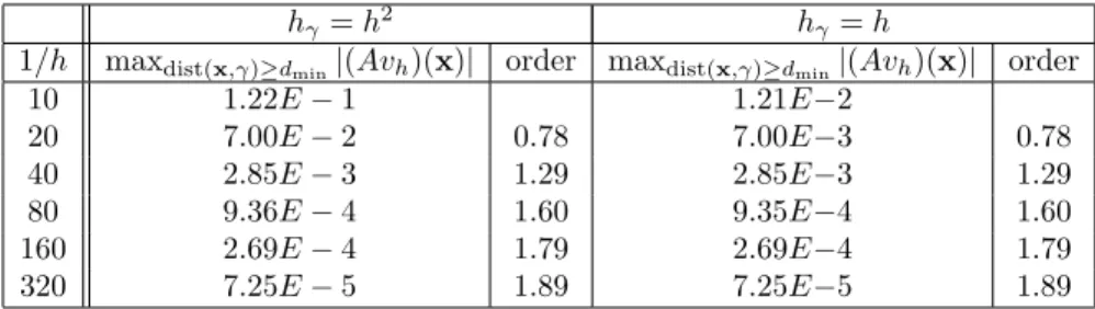
In the second test, we compute the value max
dist(x,γ)≥dmin
|(Av
h)(x) |
with the choice of h
γ= h and h
γ= h
2. Here we chose ϵ = 1/2 in d
min= max {3h, h
(4−ϵ)/4}. The two choices of h
γgive almost identical result. Base on this observation, we suggest to use more practical h
γ= h. We note that the grid size h used in our experiments gives d
min= 3h because 3h > h
(4−ϵ)/4). We can also observe with a more practical d
min= ch with c > 1, the values of max
dist(x,γ)≥dmin|(Av
h)(x) | follow O(h
2) as h gets smaller.
Table 2. Values of (Av
h)(x) for dist(x, γ) ≥ d
minwith h
γ= h and h
γ= h
2.
h
γ= h
2h
γ= h
1/h max
dist(x,γ)≥dmin|(Av
h)(x) | order max
dist(x,γ)≥dmin|(Av
h)(x) | order
10 1.22E − 1 1.21E−2
20 7.00E − 2 0.78 7.00E−3 0.78
40 2.85E − 3 1.29 2.85E−3 1.29
80 9.36E − 4 1.60 9.35E −4 1.60
160 2.69E − 4 1.79 2.69E −4 1.79
320 7.25E − 5 1.89 7.25E −5 1.89
In the following we compare our approach and the IB method for various γ. Based on the previous observation of errors with more practical choices of h
γand d
min, we use those more practical values in our experiments. First we consider the following model problem with γ, a circle centered at the origin and with its radius 0.5,
−△u(x, y) = δ(γ, (x, y)), (x, y) ∈ Ω, u(x, y) = 1 − log(2 √
x
2+ y
2)/2, (x, y) ∈ ∂Ω,
(5.1)
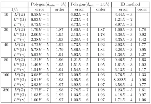
Table 3. Example 1: Numerical errors for the solution of the radially symmetric singular Poisson equation using the new method and the immersed boundary method.
Polygon(d
min= 3h) Polygon(d
min= 1.5h) IB method
1/h error order error order error order
10 L
2(Ω) 6.58E − 4 6.62E − 4 3.44E − 3
L
∞(Ω) 6.93E − 4 7.23E − 4 1.21E − 2
L
∞(γ) 8.72E − 4 8.73E − 4 8.97E − 3
20 L
2(Ω) 1.79E − 4 1.87 1.80E − 4 1.87 1.00E − 3 1.78 L
∞(Ω) 2.00E − 4 1.95 2.10E − 4 1.78 6.38E − 3 0.92 L
∞(γ) 2.28E − 4 1.93 2.28E − 4 1.93 3.35E − 3 1.42 40 L
2(Ω) 4.72E − 5 1.92 4.73E − 5 1.92 2.93E − 4 1.77 L
∞(Ω) 5.78E − 5 1.79 5.86E − 5 1.84 3.28E − 3 0.95 L
∞(γ) 5.92E − 5 1.94 5.93E − 5 1.94 1.38E − 3 1.27 80 L
2(Ω) 1.21E − 5 1.96 1.21E − 5 1.96 9.46E − 5 1.63 L
∞(Ω) 1.49E − 5 1.95 1.51E − 5 1.95 1.61E − 3 1.02 L
∞(γ) 1.54E − 5 1.94 1.54E − 5 1.94 6.13E − 4 1.17 160 L
2(Ω) 3.08E − 6 1.97 3.09E − 6 1.96 3.76E − 5 1.33 L
∞(Ω) 3.91E − 6 1.93 3.95E − 6 1.93 8.222E − 4 0.96 L
∞(γ) 3.93E − 6 1.97 3.92E − 6 1.97 3.58E − 4 0.77 320 L
2(Ω) 7.77E − 7 1.98 7.78E − 7 1.98 1.23E − 5 1.61 L
∞(Ω) 1.03E − 6 1.92 1.03E − 6 1.93 4.18E − 4 0.97 L
∞(γ) 1.00E − 6 1.97 1.00E − 6 1.97 1.71E − 4 1.06
0 5e-05 0.0001 0.00015 0.0002 0.00025
-0.8-1 -0.4-0.6 0-0.2 0.4 0.2 0.8 0.6 1
-1 -0.8-0.6 -0.4-0.2 0 0.2 0.4 0.6 0.8 1 0 0.001 0.002 0.003 0.004 0.005 0.006 0.007
-1-0.8-0.6-0.4-0.2 0 0.2 0.4 0.6 0.8 1 -1-0.8
-0.6-0.4 -0.2 0 0.2
0.4 0.6 0.8 1
Figure 3. Plot of |u − U
h| from the new method(left) and the IB method(right) with 1/h = 20.
which gives the exact solution u(x, y) =
{ 1, for x
2+ y
2≤ 1/4
1 − log(2 √
x
2+ y
2)/2, for x
2+ y
2≥ 1/4.
In our approach, the force term is computed by using v
h(x) =
∫
γhγ
log |x − x(s)| dx(x),
where γ
hγis a polygon with its side length h
γ, which approximates γ. In the IB methods, the force term is computed by approximating the Dirac delta distribution with a piecewise linear nodal basis function, see [10]. Other choices of basis functions give similar results. In Table 3, the errors from the two methods are presented. For the case when γ is a circle, our approach gives the second order of maximum errors and L
2-errors in Ω and gives the second order of maximum errors around the interface γ. The IB method only gives the first order of the maximum errors and gives about one and half order of L
2-errors in Ω. We note that such error behaviors are consistent with those appeared in previous studies of IB methods [10]. In addition, our method with more practical d
min= 1.5h produces approximate solutions of which errors are almost identical to those from d
min= 3h.
In Figure 3, the errors from the two approaches are plotted for 1/h = 20.
In the IB method, the errors are concentrated around γ and highly oscillatory.
On the other hand, our method gives the errors which are spread over the whole domain and smooth. Based on this observation we can see that our approach eliminates bad patterns of errors and provides a more sound way for approximating the singular force term.
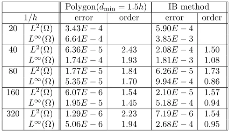
Table 4. Example 2-1: Numerical errors for the solution of the radially symmetric singular Poisson equation with γ, an ellipse with a = 0.2 and b = 0.3, using the new method and the immersed boundary method.
Polygon(d
min= 1.5h) IB method
1/h error order error order
20 L
2(Ω) 3.43E − 4 5.90E − 4 L
∞(Ω) 6.64E − 4 3.85E − 3 40 L
2(Ω) 6.36E − 5 2.43 2.08E − 4 1.50
L
∞(Ω) 1.74E − 4 1.93 1.81E − 3 1.08
80 L
2(Ω) 1.77E − 5 1.84 6.26E − 5 1.73
L
∞(Ω) 5.35E − 5 1.70 9.94E − 4 0.86
160 L
2(Ω) 6.07E − 6 1.54 2.10E − 5 1.57
L
∞(Ω) 1.95E − 5 1.45 5.18E − 4 0.94
320 L
2(Ω) 1.29E − 6 2.23 7.19E − 6 1.54
L
∞(Ω) 5.06E − 6 1.94 2.68E − 4 0.95
Table 5. Example 2-2: Numerical errors for the solution of the radially symmetric singular Poisson equation with γ, an ellipse with a = 0.2 and b = 0.4, using the new method and the immersed boundary method.
Polygon(d
min= 1.5h) IB method
1/h error order error order
20 L
2(Ω) 2.16E − 4 6.18E − 4 L
∞(Ω) 4.77E − 4 3.85E − 3 40 L
2(Ω) 7.41E − 5 1.54 2.06E − 4 1.58
L
∞(Ω) 1.97E − 4 1.27 1.84E − 3 1.06 80 L
2(Ω) 2.63E − 5 1.49 6.38E − 5 1.69 L
∞(Ω) 7.88E − 5 1.32 9.18E − 4 1.00 160 L
2(Ω) 5.65E − 6 2.21 2.17E − 5 1.55 L
∞(Ω) 2.04E − 5 1.94 5.39E − 4 0.76 320 L
2(Ω) 1.43E − 6 1.98 7.48E − 6 1.53 L
∞(Ω) 5.62E − 6 1.85 2.64E − 4 1.02
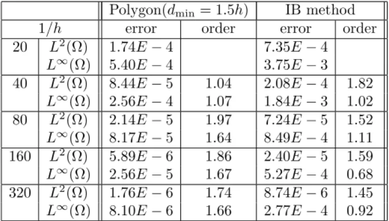
Table 6. Example 2-3: Numerical errors for the solution of the radially symmetric singular Poisson equation with γ, an ellipse with a = 0.2 and b = 0.6, using the new method and the immersed boundary method.
Polygon(d
min= 1.5h) IB method
1/h error order error order
20 L
2(Ω) 1.74E − 4 7.35E − 4 L
∞(Ω) 5.40E − 4 3.75E − 3 40 L
2(Ω) 8.44E − 5 1.04 2.08E − 4 1.82
L
∞(Ω) 2.56E − 4 1.07 1.84E − 3 1.02 80 L
2(Ω) 2.14E − 5 1.97 7.24E − 5 1.52 L
∞(Ω) 8.17E − 5 1.64 8.49E − 4 1.11 160 L
2(Ω) 5.89E − 6 1.86 2.40E − 5 1.59 L
∞(Ω) 2.56E − 5 1.67 5.27E − 4 0.68 320 L
2(Ω) 1.76E − 6 1.74 8.74E − 6 1.45 L
∞(Ω) 8.10E − 6 1.66 2.77E − 4 0.92
We consider the model problem
−△u(x, y) = δ(γ, (x, y)), (x, y) ∈ Ω, u(x, y) = 1, (x, y) ∈ ∂Ω,
(5.2)
-0.3 -0.2 -0.1 0 0.1 0.2 0.3 0.4 0.5 0.6
-0.3 -0.2 -0.1 0 0.1 0.2 0.3 0.4 0.5 0.6
Figure 4. An example of a nonconvex curve γ.
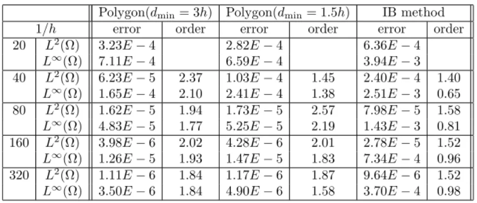
Table 7. Example 3: Numerical errors for the solution of the singular Poisson equation with γ, a nonconvex closed curve, using the new method and the IB method.
Polygon(d
min= 3h) Polygon(d
min= 1.5h) IB method
1/h error order error order error order
20 L
2(Ω) 3.23E − 4 2.82E − 4 6.36E − 4
L
∞(Ω) 7.11E − 4 6.59E − 4 3.94E − 3
40 L
2(Ω) 6.23E − 5 2.37 1.03E − 4 1.45 2.40E − 4 1.40 L
∞(Ω) 1.65E − 4 2.10 2.41E − 4 1.38 2.51E − 3 0.65 80 L
2(Ω) 1.62E − 5 1.94 1.73E − 5 2.57 7.98E − 5 1.58 L
∞(Ω) 4.83E − 5 1.77 5.25E − 5 2.19 1.43E − 3 0.81 160 L
2(Ω) 3.98E − 6 2.02 4.28E − 6 2.01 2.78E − 5 1.52 L
∞(Ω) 1.26E − 5 1.93 1.47E − 5 1.83 7.34E − 4 0.96 320 L
2(Ω) 1.11E − 6 1.84 1.17E − 6 1.87 9.64E − 6 1.52 L
∞(Ω) 3.50E − 6 1.84 4.90E − 6 1.58 3.70E − 4 0.98
where γ is an ellipse,
γ : x
2a
2+ y
2b
2= 1,
with its major radius a and minor radius b. Since the analytic form of u(x, y) is not known, at the grid level h we approximate the errors by computing
error ≈ ∥U
2h− U
h∥
∥U
h∥ ,
where U
hdenotes the approximated solution with the given grid size h and
∥ · ∥ denotes a norm considered. In Tables 4-6, the errors are presented for
aspect ratios, b/a = 1.5, 2, and 3. As the aspect ratio gets larger, the order of
accuracy becomes lower. The loss of order of accuracy is also observed for the
IB method. We note that the ellipse γ with a bad aspect ratio does not satisfy
Assumption 4.1. In spite of the lost of accuracy for the bad aspect ratio of γ,
our approach still provides much more accurate approximations than the IB method.
As our last numerical example, we consider the model problem (5.2) with a nonconvex interface, see Figure 4,
γ : (x(θ), y(θ)) = (r(θ) cos(θ), r(θ) sin(θ)), 0 ≤ θ ≤ 1, where
r(θ) = 0.5(sin
3θ + cos
3θ).
Here we observe loss of accuracy for both our method and the IB method, which is due to the bad shape of the interface. Our approach still produces much more accurate approximations than the IB method. By selecting a larger d
min= 3h, we are able to improve the order of accuracy of our approach.
References
[1] J. T. Beale and A. T. Layton, On the accuracy of finite difference methods for elliptic problems with interfaces, Commun. Appl. Math. Comput. Sci. 1 (2006), 91–119.
[2] D. Boffi and L. Gastaldi, A finite element approach for the immersed boundary method, Comput. & Structures 81 (2003), no. 8-11, 491–501.
[3] D. Gilbarg and N. S. Trudinger, Elliptic partial differential equations of second order, Classics in Mathematics, Reprint of the 1998 edition, Springer-Verlag, Berlin, 2001.
[4] E. Givelberg, Immersed finite element method, Preprint.
[5] R. J. LeVeque and Z. L. Li, The immersed interface method for elliptic equations with discontinuous coefficients and singular sources, SIAM J. Numer. Anal. 31 (1994), no.
4, 1019–1044.
[6] A. Mayo, The fast solution of Poisson’s and the biharmonic equations on irregular regions, SIAM J. Numer. Anal. 21 (1984), no. 2, 285–299.
[7] , Fast high order accurate solution of Laplace’s equation on irregular regions, SIAM J. Sci. Statist. Comput. 6 (1985), no. 1, 144–157.
[8] C. S. Peskin, Numerical analysis of blood flow in the heart, J. Computational Phys. 25 (1977), no. 3, 220–252.
[9] , The immersed boundary method, Acta Numer. 11 (2002), 479–517.
[10] A.-K. Tornberg and B. Engquist, Numerical approximations of singular source terms in differential equations, J. Comput. Phys. 200 (2004), no. 2, 462–488.
[11] , Regularization techniques for numerical approximation of PDEs with singular- ities, J. Sci. Comput. 19 (2003), no. 1-3, 527–552.
[12] L. Zhang, A. Gerstenberger, X. Wang, and W. K. Liu, Immersed finite element method, Comput. Methods Appl. Mech. Engrg. 193 (2004), no. 21-22, 2051–2067,
Department of Applied Mathematics Kyung Hee University
Yongin 446-701, Korea
E-mail address: [email protected], [email protected]