Vol. 21, No. 2, pp. 27-34, April 2017
Heave Compensation System Design for Offshore Crane based on Input-Output Linearization
Nhat-Binh Le*, Byung-Gak Kim* and Young-Bok Kim*†
(Received 18 November 2016, Revision received 14 February 2017, Accepted 14 February 2017)
Abstract: A heave motion of the offshore crane system with load is affected by unpredictable external factors. Therefore the offshore crane must satisfy rigorous requirements in terms of safety and efficiency.
This paper intends to reduce the heave displacement of load position which is produced by rope extension and sea wave disturbance in vertical motion. In this system, the load position is compensated by the winch actuator control. The rope is modeled as a mass-damper-spring system, and a controller is designed by the input-output linearization method. The model system and the proposed control method are evaluated on the simulation results.
Key Words:Rope dynamics, Offshore crane, Heave compensation, Input-output linearization.
*†Young-Bok Kim(corresponding author) : Department of Mechanical System Engineering, Pukyong National University.
E-mail : [email protected], Tel : 051-629-6197
*Nhat-Binh Le and Byung-Gak Kim : Pukyong National University.
1. Introduction
In actual operation, the harsh sea conditions are included such as sea wave, rope extension, wind and tidal, etc. Under the harsh sea conditions, the offshore vessel operations have a possibility of keeping the position or heading by using vessel thrusts. But the heave compensation is unachievable by control in similar method. Dealing with these challenges and difficulties, the heave compensation system is applied and illustrated with remarkable ability. In recent years, there have been many researches on the heave compensation system [1~4].
Messineo [2] presented an adaptive observer and two external models used for offshore crane
operating under the effects of heave motion.
Hatleskog and Dunnigan [4] introduced a dynamic model of compensator and drill string to simulate the vessel heaving motion, the displacement of the compensator, drill string and drill bit. However, their systems were too complex to apply to the real system. As already known, the input/output linearization and input/output decoupling method are branch of control theories approaching for nonlinear models, such that these have been widely used to enhance transient control performance [5, 6, 7, 12].
Zheng [8] presented a practical approach to disturbance decoupling control where the cross-couplings between control loops as well as the external disturbances are treated as disturbance which is estimated in real time and rejected.
A relevant study was produced by Kaldmӓe [9], Semsar [10], and Isidori [11]. Anyway, all these papers evaluated and demonstrated the good control performance of the proposed controller. When the rope is emphasized, its high flexibility and low
internal damping characteristics are considered [13, 14, 15]. The research of Moon et al. [16] presented the vertical motion control of the building facade maintenance robot with built-in guide rail. The dynamic model was required to update the spring stiffness and damping constant. However, the offshore crane is affected by many external and internal facts, such as rope extension, sea wave disturbance and etc. Even though the updating parameters is possible, it is not easy to satisfy the system stability and control performance.
Considering these facts, this paper deals with the load position control of offshore crane operated by a winch system. Because the rope parameters in mathematical model are strongly depended on changing in rope length, the spring stiffness and damping coefficient have to be calculated with time- varying process for keeping control performance and system stability. This is the key issue of this study.
Also, the input/output linearization and decoupling method are applied to this study for coping with hard system nonlinearity.
2. Mathematical modeling
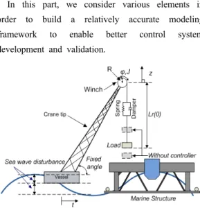
In this part, we consider various elements in order to build a relatively accurate modeling framework to enable better control system development and validation.
Fig. 1 Heave compensation system
A heave compensation system is established and shown in Fig. 1.
In this study, the offshore crane structure is modeled as a rigid body system. The main object of crane operation is moving the load in vertical direction as illustrated in Fig. 1. And, the authors assume that the crane tip angle is fixed. The winch is located at the crane tip and works as the main actuator to control the load position. The vertical rope extension due to the load moving can be approximated by the spring-mass-damper system.
The purpose of control system design is keeping the load position and tracking a desired trajectory under the disturbances such as sea wave attack and rope extension.
2.1 The equivalent mass in vertical motion
The rope mass is accumulated partly to the load and halfway to the winch when the rope is wound or released by winch system. Then an equivalent mass in vertical motion is obtained as follows:
(1)
Where denotes mass of load hung on to the end of rope, denotes the mass per meter unit rope length, denotes the nominal value of rope length, and denote the radius and angular displacement of the winch with , respectively.
2.2 Rope extension
To calculate and estimate rope extension property, the Newton/Euler method is introduced. Hence, it holds that:
(2)
In Eq. (2), denotes load acceleration,
and are rope’s dynamic spring and damping force, respectively. These dynamic forces are given as follows:
(3)
(4)
Where and denote spring stiffness and damping constant of the rope, respectively.
The load acceleration is more precisely given in Eq. (5) and exited by winch acceleration parameter . It is consisted of the second-order derivative of rope extension and second-order derivative of sea wave disturbance .
(5)
From Eqs. (2)~(5), the second-order expandable equation of can be expressed as follows:
(6)
According to Moon al at [16], the spring stiffness and damping constant of the rope can be determined by changing length of rope.
(7)
(8)
Where denote the constant of damping, Young's modulus and the intersectional area of rope, respectively. And, denotes the overall normal rope length, is given as bellows:
(9)
2.3 The winch dynamics
As mentioned already, the heave motion of crane system is controlled by a winch. In general, the dynamics of winch is obtained as follows:
(10)
Where and are inertia moment, damping coefficient, torque of the winch and tension of the rope, respectively.
The tension of rope is simply given by the spring force and damping force as follows:
(11)
2.4 Sea wave disturbance
Following Fossen’s results [12], the sea wave is described as the sum of modes and unknown term .
sin
(12)Where , and are the amplitude, period and phrase of mode , respectively.
Assume that the sea wave disturbance, second-order of sea wave disturbance are predicted.
And, it is assumed that the vertical motion of vessel is calculated also.
3. Controller design
The load position is calculated based on the Eq.
(13).
(13)
Based on Eqs. (1)~(13), the state space equation for load position can be derived. Before forming the state space equation of this nonlinear system, it is essential to define state variables. Let us define the
states as follows:
(14)
Where is the angular displacement, is angular velocity of the winch. And denotes rope extension. is derivative of is the sea wave disturbance. Lastly, is derivative of . Where the damping coefficient of the winch and damping constant of the rope extension are neglected. The state equation is created with previous kinetics equations and the state definitions of Eq. (14).
≥ (15)
Where
(16)
with
(17)The angular displacement of the winch (), the rope extension () and the sea wave disturbance () are used for feedback control. The control input of the system is the torque function of the winch.
For the vertical motion of load, the overall normal rope length which is the distance from the top of crane tip to the load position, is time-varying, and it makes the rope parameter variation.
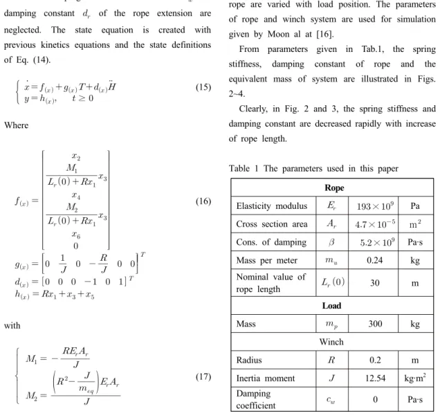
Also the equivalent mass , the spring stiffness of the rope and the damping constant of the rope are varied with load position. The parameters of rope and winch system are used for simulation given by Moon al at [16].
From parameters given in Tab.1, the spring stiffness, damping constant of rope and the equivalent mass of system are illustrated in Figs.
2~4.
Clearly, in Fig. 2 and 3, the spring stiffness and damping constant are decreased rapidly with increase of rope length.
Table 1 The parameters used in this paper Rope
Elasticity modulus × Pa Cross section area × m Cons. of damping × Pa·s Mass per meter 0.24 kg Nominal value of
rope length 30 m
Load
Mass 300 kg
Winch
Radius 0.2 m
Inertia moment 12.54 kg·m2 Damping
coefficient 0 Pa·s
Fig. 2 Spring stiffness variation with rope length
Fig. 3 Damping constant variation with rope length
Fig. 4 Mass variation with rope length
With the small changes of equivalent mass when the rope length changes as shown in Fig. 4, the approximate coefficient can be rewritten as bellows:
≃
(18)
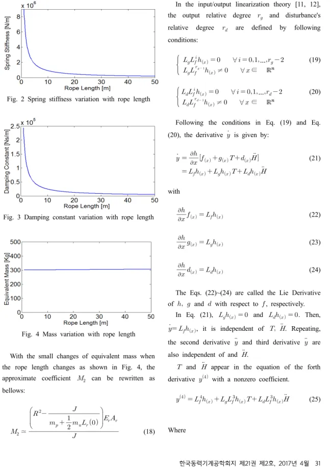
In the input/output linearization theory [11, 12], the output relative degree and disturbance's relative degree are defined by following conditions:
∀ … ≠ ∀ ∈
(19)
∀ … ≠ ∀ ∈
(20)
Following the conditions in Eq. (19) and Eq.
(20), the derivative is given by:
(21)
with
(22)
(23)
(24)
The Eqs. (22)~(24) are called the Lie Derivative of and with respect to , respectively.
In Eq. (21), and . Then,
, it is independent of . Repeating, the second derivative and third derivative are also independent of and .
and appear in the equation of the forth derivative with a nonzero coefficient.
(25)
Where
≠
(26)
≠ (27)
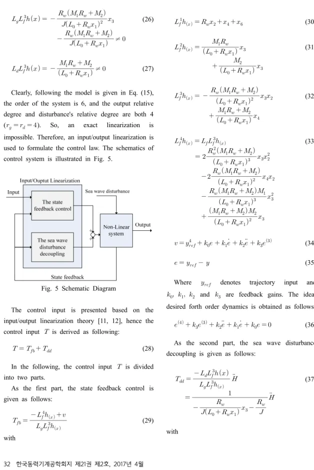
Clearly, following the model is given in Eq. (15), the order of the system is 6, and the output relative degree and disturbance's relative degree are both 4 ( ). So, an exact linearization is impossible. Therefore, an input/output linearization is used to formulate the control law. The schematics of control system is illustrated in Fig. 5.
Fig. 5 Schematic Diagram
The control input is presented based on the input/output linearization theory [11, 12], hence the control input is derived as following:
(28)
In the following, the control input is divided into two parts.
As the first part, the state feedback control is given as follows:
(29)
with
(30)
(31)
(32)
(33)
(34)
(35)
Where denotes trajectory input and
and are feedback gains. The ideal desired forth order dynamics is obtained as follows:
(36) As the second part, the sea wave disturbance decoupling is given as follows:
(37)
with
(38)
From Eqs. (28)~(38),the control input is derived as bellows:
(39)
4. Simulation results
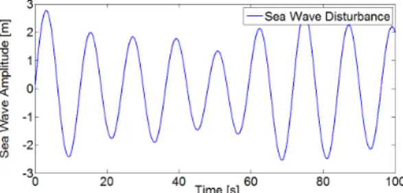
The schematics of control system in Fig. 5 is utilized in Matlab/Simulink. The parameters given in table 1 are used for simulation. The non-linear motion of vessel related sea wave disturbance is added into the simulation. Following the Eq. (12), the sea wave is described as the sum of modes and unknown term . In the simulation, the sea wave disturbance is divided into two cases for evaluating the control law as shown in table. 2. In the Fig. 7, the dotted line presents the target trajectory of the load, and the solid line is the load position when the proposed control works.
Table 2 The sea wave disturbance
Case Amplitude (m) Period (s)
1 0 ~ 5 < 10
2 0 ~ 5 > 10
Fig. 6 Sea wave disturbance : case 1
Fig. 7 Load position with disturbance : case 1
In this case, the sea wave disturbance and the rope extension are considered. Where the period of the sea wave disturbance is lower than 10 seconds.
In this simulation, the peak value of the output response is around 0.2 meter less.
Fig. 8 Sea wave disturbance : case 2
Fig. 9 Load position with disturbance : case 2
As the another case, when the period of the sea wave disturbance increases to more than 10 seconds, the controlled output shows relatively better performance than previous result in Fig. 7.
Anyway, it is clear that the proposed control system works well such that we can obtain good control performance by effectively suppressing wave disturbance etc.
5. Conclusions
This study focuses on a control system design problem with non-linear system properties such as time varying spring stiffness. After that a nonlinear control law is applied for offshore crane model with load hoisting using the input-output linearization method and decoupling strategy. Simulation results revealed that the proposed control method can greatly decrease the heave displacement as well as can accurately keep the position of load.
Acknowledgement
This work was supported by the National Research Foundation of Korea (NRF) grant funded by the Ministry of Education in Korea. (No.
NRF-2015R1D1A1A09056885)
References
1. U. A. Korde, 1998, "Active heave compensation on drill-ships in irregular waves", Ocean Engineering, Vol. 25, pp. 541-561.
2. S. Messineo and A. Serrani, 2009, "Offshore crane control based on adaptive external models", Automatica, Vol. 45, pp. 2546-2556.
3. S. I. Sagatun, 2002, "Active control of underwater installation", IEEE Transactions on Control System Technology, Vol. 10, pp.
743-748.
4. J. T. Hatleskog and M. W. Dunnigan, 2007,
"Passive compensator load variation for deep-water drilling", IEEE Journal of Oceanic Engineering, Vol. 32, pp. 593-602.
5. H. Nijmeijer and A. J. Schaft, 1990, "Nonlinear dynamical control systems", Springer-Verlag:
Berlin, Germany, pp. 172–198.
6. J. J. E. Slotine and W. Li, 1991, "Applied Nonlinear Control", Prentice-Hall: NY, USA, pp.
112–137.
7. H. A. B. TeBraake, J. V. Can, J. M. A.
Scherpen and H. B. Verbruggen, 1998, "Control of nonlinear chemical processes using neural models and feedback linearization", Computers
& Chemical Engineering, Vol. 22, pp. 1113–
1127.
8. Q. Zheng, Z. Chen and Z. Gao, 2007, "A practical approach to disturbance decoupling control", Control Engineering Practice, Vol. 17, pp. 1016-1025.
9. A. Kaldmӓe and Ü. Kotta, 2014, "Disturbance decoupling by measurement feedback", IFAC Proceedings Volumes, Vol. 47, pp. 7735-7740.
10. E. Semsar, M. J. Yazdanpanah and C. Lucas, 2003, "Nonlinear control, disturbance decoupling and load estimation in HVAC systems", Conference of Control Application.
11. A. Isidori, 1987, "Lectures on nonlinear control", notes prepared for a course at Carl CranzGesellschaft.
12. T. Fossen, 1994, "Guidance and Control of Ocean Vehicles", New York: Wiley.
13. M. F. Glushko and A. A. Chizh, 1969,
"Differential equations of motion for a mine lift cable", International Applied Mechanics, Vol. 5, pp. 17–23.
14. O. A. Goroshko, 2007, "Evolution of the dynamic theory of hoist ropes", International Applied Mechanics, Vol. 43, pp. 64–67.
15. R. F. Fung and J. H. Lin, 1997, "Vibration analysis and suppression control of an elevator string actuated by a pm synchronous servo motor", Journal of Sound and Vibration, Vol.
206, pp. 399–423.
16. S. M. Moon, J. Huh, D. Hong, S. Lee and C.
S. Han, 2015, "Vertical motion control of building facade maintenance robot with built-in guide rail", Robotics and Computer-Integrated Manufacturing, Vol. 31, pp. 11-20.