An Iterative Insertion Algorithm and a Hybrid Meta Heuristic for the Traveling Salesman Problem with Time Windows

An Iterative Insertion Algorithm and a Hybrid Meta Heuristic for the Traveling Salesman Problem with Time Windows

Byung-In Kim

Department of Industrial and Management Engineering,

Advanced Product & Production Technology Center, POSTECH, Pohang 790-784, Korea

시간제약이 있는 외판원 문제를 위한 메타휴리스틱 기법

김 병 인

포항공과대학교 산업경영공학과, 제품생산기술연구소

This paper presents a heuristic algorithm for the traveling salesman problem with time windows (TSPTW). An iterative insertion algorithm as a constructive search heuristic and a hybrid meta heuristic combining simulated annealing and tabu search with the randomized selection of 2-interchange and a simple move operator as an improving search heuristic are proposed. Computational tests performed on 400 benchmark problem instances show that the proposed algorithm generates optimal or near-optimal solutions in most cases. New best known heuristic values for many benchmark problem sets were obtained using the proposed approach.

Keywords: Traveling Salesman Problem With Time Windows (TSPTW), Simulated Annealing, Tabu Search, Meta heuristic, Iterative Insertion Algorithm

1. Introduction

The traveling salesman problem with time windows (TSPTW) is an extension of the well known traveling salesman problem (TSP) in which each city (or cus- tomer or stop) is associated with a time interval [earliest visit time, latest visit time], called a time window. Each customer must be visited exactly once and within the time window. The salesman can arrive at a customer before the customer’s earliest visit time and wait until the beginning of the window, but he or she cannot visit the customer after the customer’s lat- est visit time. Minimizing the total traveling time and minimizing the completion time, which includes wait- ing time at the customers, are the two main objective functions considered in the literature. In this paper, the

former is considered in order to compare our algo- rithm with other methods. A mathematical program- ming model for TSPTW is presented in Calvo (2000).

The TSPTW has various practical applications in- cluding package delivery, school bus routing, di- al-a-ride, and automated guided vehicle/overhead hoist transport scheduling. It is also a sub-problem of the vehicle routing problem with time windows (VRPTW) when a cluster-first, route-second approach is used.

The TSPTW is known as a hard problem to solve.

Savelsbergh (1985) constructs an instance of TSPTW from an instance of the 3-partition problem and proves that even finding a feasible solution is an NP-Complete problem. Thus, exact methods are limited to instances of small numbers of customers and narrow time windows.

In this paper, an iterative insertion algorithm, and a

†Corresponding author : Byung-In Kim, Department of Industrial and Management Engineering, POSTECH, San 31 Hyoja-dong Nam-gu Pohang 790-784, Korea, Tel：+82-54-279-2371, Fax：+82-54-279-2870, E-mail：[email protected]

Received June 2006; revision received September 2006; accepted October 2006.

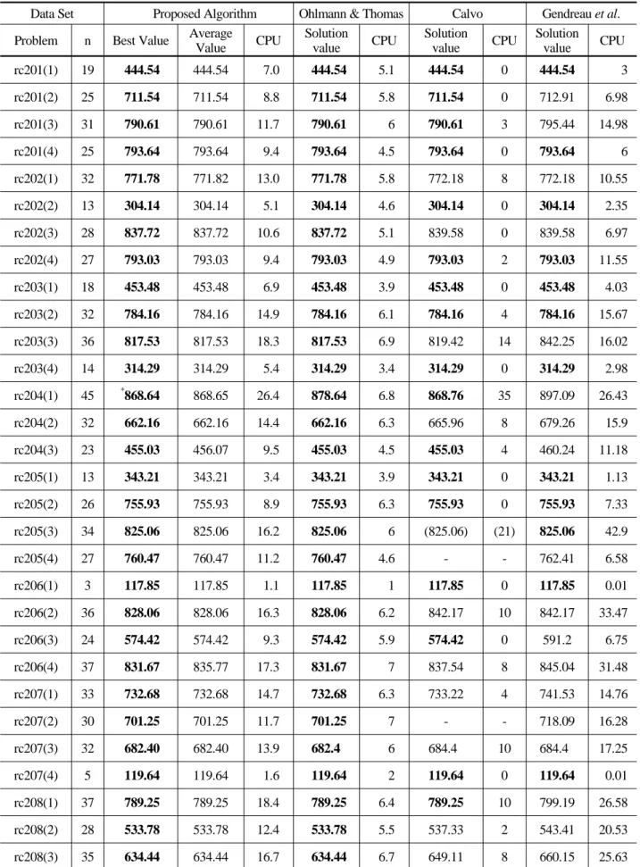
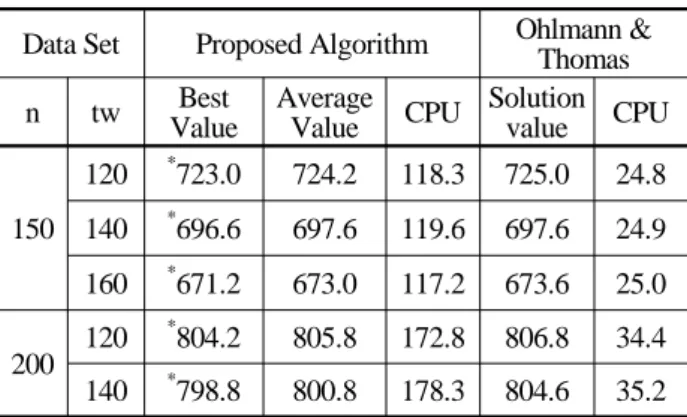
hybrid meta heuristic combining simulated annealing and tabu search with 2-interchange and a simple move operator are proposed for the TSPTW. Computational tests performed on 97 benchmark problem sets con- sisting of 400 benchmark problem instances show that the proposed approach generates optimal or near-opti- mal solutions for all the problems in reasonable com- puting time. Using the proposed approach, new best known heuristic values for 17 benchmark problem sets are obtained, and the results for 72 problem sets match the previous best known solutions. The proposed ap- proach performs particularly well on instances with large numbers of customers and wide time windows compared with the previous approaches.

This paper is organized as follows. After we briefly review the related literature on algorithms for the TSPTW in section 2, an iterative insertion algorithm is presented in section 3. A hybrid meta heuristic com- bining simulated annealing and tabu search with 2-in- terchange and a simple move operator is described in section 4. Section 5 shows the computational results on the benchmark problem sets, and section 6 provides concluding remarks.

2. Literature Review

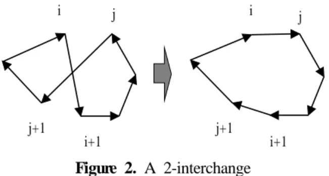
Savelsbergh (1985) proposes methods to handle time windows without increasing computational complexity for 2-interchange and Or-interchange local searches.

He also proposes an insertion algorithm which inserts the stops with tight time windows first and then the re- maining stops. Langevin et al. (1993) present a two- commodity flow model for the traveling salesman problem. They use a branch-and-bound scheme with lower bounds obtained by the LP relaxation of the two-commodity flow model and subtour elimination constraints. They find optimal solutions for problems with up to 60 nodes.

Dumas et al. (1995) propose three time window re- lated elimination tests to reduce the state space and the number of state transitions of forward dynamic pro- gramming for TSPTW. Optimal solutions are found with up to 200 nodes with narrow time windows in about a minute but they experience memory problems due to the dimensionality of their state spaces. The state spaces of their algorithm grow exponentially with respect to time window width.

Gendreau et al. (1992) propose an insertion algo- rithm and a post optimization method called GENIUS for TSP, in which a partial sequence of an existing route may be changed when a stop is inserted. Gendreau et al. (1998) apply the GENIUS algorithm to TSPTW.

While stops are inserted in the route in random order for the TSP in Gendreau et al. (1992), stops are insert- ed with non-decreasing time window widths for the TSPTW in Gendreau et al. (1998). The insertion posi- tion of a stop is determined based on a certain number of stops close to the stop with respect to the geometric distance and a certain number of stops closest to the stop with respect to the time window proximity. The post optimization consists of successive removal and reinsertion of all the stops in a route.

Calvo (2000) formulates a relaxed assignment prob- lem (AP) from the TSPTW and attempts to get a sol- ution close enough to a feasible solution of the original problem. As the objective function of the relaxed AP, he uses a weighted sum of the total travel time and the total maximum possible waiting time. After solving the relaxed AP, all the sub tours, if any, are inserted one by one into the main route. He proposes a local search method in which two objective functions (travel time and route duration) are alternated to explore the search area and a 3-opt exchange operator is used.

Carlton and Barnes (1996) present a reactive tabu search with a move operator that removes a stop and places it at a different position. They allow infeasible solutions with penalty in their search procedure. Nanry and Barnes (2000) extend this method and apply it to the pickup and delivery problem with time windows (PDPTW). They first construct an initial feasible sol- ution with a simple predecessor-successor pair in- sertion algorithm. Then, the initial solution is altered by move neighborhood search operators. Infeasible solutions are allowed with penalty during the search.

Depending on the tightness of time windows, different neighborhood search strategies are selected in their method.

Ohlmann and Thomas (2006) propose a variant of a

simulated annealing heuristic in which a penalty multi-

plier is used for infeasible solutions in addition to the

traditional temperature of the simulated annealing app-

roach. For the local search method, the 1-opt neigh-

borhood scheme is used. They obtain new best values

for many benchmark instances. 400 benchmark prob-

lem instances collected from the literature are hosted

on their homepage.

3. Iterative Insertion Algorithm for Initial Solution

Because getting a feasible solution from an infeasible solution is not an easy task, we choose to find an ini- tial feasible solution and keep the feasibility through our improvement search procedures rather than allow- ing infeasible solutions in the search process. Note that Ohlmann and Thomas (2006) allow infeasible sol- utions in their search process and have experienced several cases in which their approach could not find a feasible solution. Calvo (2000) also experienced sev- eral infeasible instances.

The proposed iterative insertion algorithm is a repet- itive procedure. As a base insertion procedure, Solo- mon (1987)’s well-known insertion algorithm is used.

Solomon’s insertion heuristic initializes a route with the farthest stop from the depot and inserts stops into the route one at a time in a serial manner. For each step, all the unrouted stops are tested for insertion at all the possible positions in the route, and the best unrouted stop and its best position are selected. A de- tailed description of this method is presented in Solo- mon (1987).

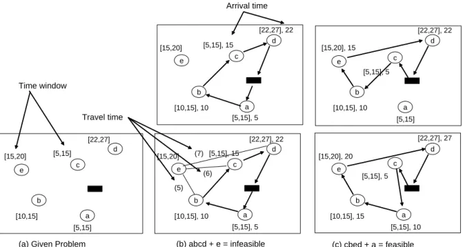
Although the Solomon’s insertion algorithm is very intuitive and robust, its performance is highly sensitive to the sequence of insertion because an insertion af- fects all subsequent insertions. For example, given

stops a,b,c,d,e, and depot, there might be a case in which stop e cannot be inserted into the route de- pot-a-b-c-d – depot while stop a can be inserted into the route depot-c-b-e-d-depot to make a new extended route depot-c-a-b-e-d-depot as shown in <Figure 1>.

In fact, the pure insertion method could not find a fea- sible solution for 26 benchmark instances, as pre- sented in section 5.1. Most sequential insertion heu- ristics have this sensitivity problem. Considering this observation, we develop an iterative insertion algo- rithm as follows.

The basic idea of the proposed approach is to insert

‘hard’ stops first and then to insert the remaining stops. Initially (at step 0), all the stops are classified as class 1, which means ‘not hard’, and are inserted into a route using Solomon’s insertion algorithm (step 11). If some stops remain unrouted after the insertion proce- dure, the procedure attempts to reduce the total travel time with a greedy 2-opt algorithm, make buffer time for the unrouted stops (step 14) and reinsert them (step 11). If some stops still remain unrouted, it attempts to maximize the total time window order count with the greedy 2-opt (step 15), which is defined later, and re- insert them (step 11). If there are unrouted stops and no additional stops can be inserted in two consecutive iterations, the remaining stops are classified as ‘hard’

stops, their class is set to 0 (step 13), the status of all the stops is set to unrouted, and the procedure is re- started (step 1).

a b

e c

d d

e c

b

a a

d e c

b a

b

e c

d

a

e c

d

b

[22,27], 22 [5,15], 15

[15,20] (7) (6) (5)

[10,15], 10

[5,15], 5

(b) abcd + e = infeasible (c) cbed + a = feasible (a) Given Problem

[10,15]

[5,15]

[5,15]

[15,20]

[22,27]

Travel time Time window

[5,15], 5 [10,15], 10

[5,15], 15 [15,20]

[22,27], 22

[10,15], 10

[5,15]

[5,15], 5 [15,20], 15

[22,27], 22

[10,15], 15

[5,15], 10 [22,27], 27

[5,15], 5 [15,20], 20

Arrival time

Figure 1. Sensitivity of an insertion algorithm to the sequence of insertion.

<Iterative insertion algorithm>

Step 0: Set status of all the stops = unrouted, class of stops = 1 Initialize a route with a path depot-depot.

Step 1: Repeat steps 2 – 16 until a termination criterion is reached.

Step 2: If there are stops whose class = 0, Step 3: Set improve_type = 1.

Step 4: Insert unrouted stops whose class = 0 using Solomon’s insertion procedure into the route.

Set the status of stops inserted = routed.

Step 5: If all the stops whose class = 0 are routed, go to step 9.

Step 6: If there are unrouted stops with class = 0 and no additional stops can be inserted in two consecutive trials, stop the procedure.

No feasible solution is found.

Step 7: If improve_type = 1,

Improve the route constructed with greedy 2-opt heuristic with objective minimizing the total travel time.

Set improve_type = 2.

Go to step 4.

Step 8: Otherwise,

Improve the route constructed with greedy 2-opt heuristic with objective maximizing the total time window order.

Set improve_type = 1.

Go to step 4.

Step 9: If there are stops whose class = 1, Step 10: Set improve_type = 1.

Step 11: Insert unrouted stops using Solomon’s insertion procedure into the route.

Set the status of stops inserted = routed.

Step 12: If all the stops whose class = 1 are routed, stop the procedure.

A feasible solution is found.

Step 13: If there are unrouted stops and no additional stops can be inserted in two consecutive trials, Set the class of unrouted stops = 0.

Reinitialize a route with a path depot-depot.

Set the status of all the stops = unrouted.

Go to step 2.

Step 14: If improve_type = 1,

Improve the route constructed with greedy 2-opt heuristic with objective of minimizing the total travel time.

Set improve_type = 2.

Go to step 11.

Step 15: Otherwise,

Improve the route constructed with greedy 2-opt heuristic with objective of maximi- zing the total time window order.

Set improve_type = 1.

Go to step 11 Step 16: Otherwise,

Stop the procedure. A feasible solution is found.

Now the stops classified as ‘hard’ stops (class = 0 ) are routed first (steps 2 through 8). The steps are sim- ilar to the previous ones except step 6. In step 6, if

there are unrouted stops whose class is 0 and no addi-

tional stops can be inserted in two consecutive iter-

ations, the procedure stops with infeasibility. Steps

2-16 are iterated until a feasible solution is found or until the procedure cannot insert any of ‘hard’ stops in step 6.

The greedy 2-opt uses the 2-interchange operator. It exchanges two links of a route as shown in <Figure 2>. Two links (i, i+1) and (j, j+1) are replaced with (i, j) and (i+1, j+1) and the orientation of the path (i+1,

… , j) is reversed. A solution is said to be 2-opt if it is impossible to improve it by exchanging a link with an- other link. The 2-opt algorithm considers all the possi- ble exchanges and selects the best exchange as a per- manent move at each step, while the greedy 2-opt al- gorithm makes a permanent move whenever it finds an improving move. Because greedy 2-opt typically re- quires less computational time, it is used in our approach.

i j i j

i+1

j+1 j+1

i+1 Figure 2. A 2-interchange

Two alternative objective functions are used for the greedy 2-opt algorithm in the proposed approach.

First, the total travel time is minimized. When no stops can be inserted into a route optimized with regard to the total travel time, however, maximizing the total time window order count is used as an alternative function. The time window order count is defined as the total number of stop pairs whose sequence orders in the route match with their time windows. For exam- ple, when stop i with time window [e

(earlist visit time), l

(latest visit time)] is sequenced before stop j with time window [e

, l

] in a route, if e

≤ e

and l

≤ l

the stop pair is well sequenced with regard to their time windows thus, it has 1 time window order count.

If the conditions do not match, the pair does not have a time window order count. <Figure 1>shows two ex- amples. While the partial route of <Figure 1-(b) top>, depot-a-b-c-d-depot, has time window order count of 5(ab, ac, ad, bd, and cd), the one of <Figure 1-(c) top>, depot-a-c-b-d-depot, has 6 (ac, ab, ad, cb, cd, and bd).

Note that the route of the former has better total travel time compared with the latter but the latter has better total time window order count. While stop e cannot be

inserted in the former route, the stop can be inserted into the latter route.

Using the proposed approach, we could find a fea- sible solution for each of the 400 benchmark problem instances.

4. A Hybrid Improvement Meta Heuristic Approach

In addition to the 2-interchange operator described in the previous section, a simple move operator is used as a neighborhood search operator in our improvement procedure. The simple move operator replaces stop i such that it will be visited right after stop j as shown in

<Figure 3>. After experimenting with other operators such as the CROSS exchange of Taillard et al. (1997) and the Or-interchange of Or (1976), we decided to use the 2-interchange and the simple move operator due to their effectiveness and short computation time.

i-1 i+1 i-1 i+1

j-1

j j+1 j-1

j j+1

i i

Figure 3. A simple move operator

A hybrid meta heuristic of simulated annealing and tabu search with the two operators is proposed below.

The basic framework of the proposed approach fol- lows a typical simulated annealing (SA) algorithm.

Our approach varies from others in using tabu list within SA and using random selection of move oper- ators at each iteration.

Step 0 of the algorithm is an initialization step in which an initial feasible solution S

is obtained through the iterative insertion algorithm and the parameters are set. The function f(.) represents an objective function.

In this research, the total travel time is used as the ob-

jective function. The initial temperature in step 0 is set

such that solutions with (100*2/number of stops) per-

cent longer travel time than the initial solution are like-

ly to be accepted with 25 percent probability. For ex-

ample, when the number of stops in a route is 20,

(100*2/number of stops) percent becomes 10 percent

< Hybrid Meta heuristic algorithm >

Step 0: Get a feasible initial solution S

using the iterative insertion algorithm.

Set initial temperature T = (-(2/num of stops) *f(S

) / ln(0.25) Get the number of maximum temperature changes Niter (=30) Get the number of iterations per temperature

Nover ( = min(1000000, num of stops*10000))

Get the maximum number of solutions evaluated per temperature Nlimit ( = min(200000, num of stops*1000))

Get the cooling coefficient  ( = 0.925)

Get the tabu tenure l ( = min(100, num of stops* num of stops/2)) Set the best solution S

= S

Set the global best solution S

= S

Set iteration count k =1

Step 1: Repeat steps 2 – 18 while k ≤ Niter Step 2: Set current solution S

= S

Initialize tabu list tabu[][] = 0 Initialize tabu list obj_tabu_list[] = 0 Step 3: Set inner iteration count m = 1

Set evaluated count n = 0

Step 4: Repeat steps 5-17 while m ≤ Nover and n ≤ Nlimit

Step 5: Generate sequence indices i, j randomly and get corresponding stop indices stop_i, stop_j Step 6: Select randomly the 2-interchange operator or the simple move operator with equal chance Step 7: If selected operator = 2-interchange and tabu [stop_i][stop_j] ≤ m

or selected operator = simple move and tabu[stop_j][stop_i] ≤ m Step 8: Calculate f(S

) using the operator and stop indices selected Step 9: Calculate travel time difference △ = f(S

)- f(S

)

Step 10: If obj_tabu_list[f(S

)] ≤ m and ( △ <0 or ( △≥ 0 and rand(0,1)< e

)), Step 11: Set obj_tabu_list[obj_value] = m + 100

Increment n by 1 Step 12: Check feasibility of S

If S

is feasible,

Step 13: Set S

= S

If selected operator = 2-interchange, Set tabu[stop_i][stop_j] = m+l Otherwise,

Set tabu[stop_j][stop_i] = m+l Step 14: If f(S

) ≤ f(S

),

Set S

= S

Step 15: Improve S

using 2-opt improvement Step 16: If f(S

) ≤ f(S

), Set S

= S

Step 17: Increment m by 1

Step 18: Set T =  *T, Increment k by 1

and when the number of stops is 200, it is 1 percent.

The two numbers, (2/number of stops) and 25 percent, were selected intuitively and verified experimentally.

The other parameters set in step 0 were also estab- lished through pre experimental tests. The number of stops of a problem is took into consideration in most

parameters to adjust the computing time dynamically according to the problem size.

At each temperature value, the current solution is re-

placed with the current best solution and the two di-

mensional tabu list and the tabu list for objective value

are initialized (step 2). The tabu list, tabu[stop_i][s-

top_j], determines when any specific two stops (stop_i and stop_j) must not be considered for the move operators. The upper-right corner elements of the tabu list, i.e., stop_i <stop_j, keep the tabu period for the 2-interchange, while the lower-left corner elements keep the tabu period for the simple move operator.

The tabu list, obj_tabu_list[objective value] keep the tabu period for the objective value.

At each inner-iteration, sequence indices i and j are randomly selected (step 5). The sequence index repre- sents the order of visits in a route. Thus, if there are 5 stops in a route, the possible sequence indices are 1, 2, 3, 4, and 5. Each sequence index has a corresponding stop index. For example, when a route solution has a sequence of stops 31, 20, 45, 4, 27, and the sequence indices selected are 2 and 4, their corresponding stop indices are 20 and 4.

In order to diversify the search area, the 2-inter- change operator or the simple move operator is se- lected randomly with equal probability at each iter- ation (step 6). Depending on the selected operator, the upper-right corner or lower-left corner of the tabu list is checked (step 7) and, when the intended move is not in the tabu list, i.e., the tabu tenure of the pair is al- ready past, the move is further considered. In step 8, the total travel time of the solution newly obtained by the move operator is calculated. In this step, only af- fected portions of the solution are considered. In

<Figure 2>, the total travel time of the right hand sol- ution is calculated by the travel time of the left hand solution f(S

) plus travel time (i, j) plus travel time (i+1, j+1) minus travel time (i, i+1) minus travel time (j, j+1). Note that we are assuming a symmetric TSPTW such that the travel time for path (i+1, … , j) is the same as the travel time for path (j, … , i+1).

Similarly, the total travel time for the new solution constructed by the simple move operator is easily calculated. Then, the difference between the newly constructed solution and the current solution is calcu- lated (step 9).

When the new solution value f(S

) is not in the ob- jective value tabu list and if the move is an improve- ment, the feasibility of the solution S

is checked.

When the move is not in improving direction, the fea- sibility of the solution S

is checked with a proba- bility e

(step 10). When the solution S

is feasible with the time window constraints (step 12), the current solution is replaced with the new solution, and the tabu list is updated (step 13). When the solution S

is better than the current best solution S

, the best sol-

ution is also updated (step 14). The best solution is further improved using the 2-opt improvement algo- rithm (step 15). When the improved solution is better than the global best solution, the global best solution is updated accordingly (step 16). The steps are iterated for the given number of iterations. The global best sol- ution will be the final solution.

5. Computational Results

The algorithms were tested on 400 TSPTW bench- mark problem instances taken from the literature: 70 instances from Langevin et al. (1993), 135 from Dumas et al. (1995), 30 from Potvin and Bengio (1996), 140 from Gendreau et al. (1998), and 25 from Ohlmann and Thomas (2006). Ohlmann and Thomas (2006) have collected the data sets and made them available from http://myweb.uiowa.edu/bthoa/TSPTWBenchmarkData Sets.htm.

All the data sets except the data set of Potvin and Bengio (1996) are classified by the number of custom- ers and time window width. Each class of problems of Dumas et al. (1995), Gendreau et al. (1998), and Ohlmann and Thomas (2006) has five instances, while each class of Langevin et al. (1993) has ten instances for each data set of customer number – time window width pair. Thus, the results reported on those data sets are the averages over five instances or ten instances. Potvin and Bengio (1996) generated individual TSPTW in- stances from Solomon’s RC2 VRPTW instances.

The algorithms were implemented in the C langu- age. Computational times in this section are in seconds on a Windows XP Pentium 4, 3.4 GHz processor with 3.25 GB of RAM, and include the times for initial sol- ution generation and improvement steps. The comput- ing times of other algorithms are from the reference papers.

5.1 Effectiveness of the Iterative Insertion Algorithm for Initial Solution

<Table 1> shows the effectiveness of the proposed

iterative insertion algorithm. An insertion algorithm

without iterations and the concept of classes could not

generate a feasible solution for 26 of the 400 problem

instances. The proposed iterative insertion algorithm

could produce a feasible solution for all 400. Note that

Ohlmann and Thomas (2006) could not find a feasible

solution in several trials for several problem sets (for example, the rc204(1) problem instance of Potvin and Bengio).

Table 1. Naive insertion algorithm vs. iterative in- sertion algorithm

Data set

Number of total instances

Number of infeasible instances

using naive insertion method

Number of infeasible instances

using iterative insertion method Langevin

et al. 70 6 0

Dumas

et al. 135 14 0

Potvin and

Bengio 30 5 0

Gendreau

et al. 140 1 0

Ohlmann

& Thomas 25 0 0

5.2 Effects of Tabu List and Move Operators In order to examine the effects of the tabu list and selection of move operators within SA, 4 combinations of those factors have been tested as in <Table 2>. In the first two experiments, a move operator (either the simple move or the 2-interchange) was randomly se- lected at each iteration as described in the previous section. In the third experiment, the simple move oper- ator was used exclusively while the 2-interchange was used in the last experiment. Tabu list was used within SA for all the experiments but the second one. Com- parison of the first, third, and the last experiments shows the effectiveness of the random selection strat- egy of move operators. Random selection of move op- erators generates better solutions for all the problem sets.

Comparison of the first two experiments shows that SA with the tabu list produces better solutions for all the problem sets. We observed similar results for other data sets through our experiments. The results presented in the next subsection have been obtained by using mixed move with tabu list for all the problem sets.

5.3 Benchmark Tests

<Table 3> provides computational results for the in- stances of Langevin et al. (1993). The first column shows the number of customers in a problem instance and the second column shows the average time win- dow width. Since optimal solutions for the problems with 60 customers are only partially known, the aver- age solution values of ten instances for the exact meth- od cannot be calculated and are left blank.

We have compared the proposed algorithm to known optimal solutions and the solutions of Calvo (2000) and Ohlmann and Thomas (2006). For each instance, we provide the best solution obtained in ten runs as well as the average solutions and the average CPU time in seconds. The proposed approach produces op- timal solutions for three problem sets and matches the other algorithms for two problem sets. The last prob- lem set with 60 customers and time window 40 is 0.1 longer from the other approaches. There is one in- stance out of 10 in which the solution of the proposed approach is one unit longer than the solution of other approaches, but the proposed approach matches other approaches for the remaining nine instances. It is diffi- cult to compare computational times among the ap- proaches because of different processor speeds, mem- ory, and implementation details. However, the compu- tational time of the proposed approach is longer than

Table 2. Comparison of various strategies using instances from Ohlmann and Thomas (2006)

Mixed move with tabu Mixed move without tabu Simple move with tabu 2-interchange with tabu Solution value CPU Solution value CPU Solution value CPU Solution value CPU

724.6 126.3 740.2 30.8 727.2 112.4 727.4 119.1

697.4 118.0 718.0 33.9 698.0 111.4 698.2 122.4

671.8 117.9 701.2 29.1 675.6 108.8 678.4 119.3

806.8 176.5 823.2 46.5 812.6 166.3 807.6 168.6

801.2 185.7 814.2 46.0 804.2 179.2 806.0 175.9

Table 3. Results on instances from Langevin et al. (1993)

Data Set Exact Algorithm Proposed Algorithm Ohlmann & Thomas Calvo n tw Solution

value CPU Best Value Avg. Value CPU Solution

value CPU Solution

value CPU 20 30 724.7 0.4 724.72 724.72 4.7 724.7 2.4 724.7 0.0

40 721.5 0.7 721.55 721.55 4.8 721.5 3.4 721.5 0.0 40 20 982.4 1.7 982.71 982.71 16.4 982.7 4.4 982.7 0.3 40 951.8 7.3 951.82 951.82 17.1 951.8 4.7 951.8 0.6

60

20 - - 1215.68 1215.68 33.4 1215.7 5.6 1215.7 5.0

30 - - 1183.25 1183.25 34.2 1183.2 8.1 1183.2 5.0

40 - - 1160.90 1160.90 34.7 1160.8 9.0 1160.8 10.9 Table 4. Results on instances from Dumas et al. (1995)

Data Set Exact Algorithm Proposed Algorithm Ohlmann & Thomas Calvo n tw Solution

Value CPU Best Value Avg. Value CPU Solution

value CPU Solution

value CPU

20

20 361.2 0.0 361.2 361.2 5.7 361.2 2.0 361.2 0.0 40 316.0 0.1 316.0 316.0 6.6 316.0 2.7 316.0 0.0 60 309.8 0.1 309.8 309.8 6.8 309.8 2.5 309.8 0.0 80 311.0 0.2 311.0 311.0 6.9 311.0 3.0 311.0 0.0 100 275.2 1.3 275.2 275.2 7.3 275.2 3.2 275.2 0.0

40

20 486.6 0.1 486.6 486.6 19.2 486.6 3.8 486.6 3.0 40 461.0 0.0 461.0 461.0 19.5 461.0 5.1 461.0 3.0 60 416.4 4.4 416.4 416.4 19.5 416.4 6.0 416.4 4.8 80 399.8 7.5 399.8 399.8 20.3 399.8 6.2 399.8 5.2 100 377.0 31.4 377.0 377.0 20.5 377.0 6.6 377.0 5.6

60

20 581.6 0.2 581.6 581.6 36.2 581.6 7.2 581.6 8.4 40 590.2 0.9 590.2 590.2 36.3 590.2 8.2 590.4 17.2 60 560.0 6.8 560.0 560.0 36.5 560.0 8.5 560.0 20.2 80 508.0 46.6 508.0 508.0 36.0 508.0 8.6 509.0 18.0 100 514.8 199.8 514.8 514.8 37.3 514.8 8.8 516.4 26.2

80

20 676.6 0.4 676.6 676.6 55.8 676.6 11.3 676.6 43.4 40 630.0 2.7 630.0 630.0 56.2 630.0 11.5 630.0 69.2 60 606.4 55.3 606.4 607.2 59.1 606.4 12.0 596.5(4) 71.6 80 593.8 220.3 593.8 593.8 58.6 593.8 11.5 594.4 59.6

100

20 757.6 0.6 757.6 757.6 78.2 757.6 15.4 757.8 102.6 40 701.8 7.4 701.8 701.8 80.2 701.8 15.7 703.6 128.6 60 696.6 108.0 696.6 696.6 83.1 696.6 15.9 696.6 148.0

150

20 868.4 2.4 868.4 868.4 98.6 868.4 24.7 868.6 419.8 40 834.8 115.9 834.8 834.8 107.6 834.8 25.2 837.4 529.6 60 805.0 463.0

818.6 818.7 107.6 818.8 25.6 820.4 630.0 200 20 1009.0 6.7 1009.4 1009.4 123.7 1009.0 35.1 1010.0 1456.2

40 984.2 251.4

984.2 984.4 159.5 984.6 35.2 985.4 2105.8

Table 5. Results on instances from Gendreau et al. (1998)

Data Set Proposed Algorithm Ohlmann & Thomas Calvo Gendreau et al.

n tw Best Value Average

Value CPU Solution

value CPU Solution

value CPU Solution

value CPU

20

120 265.6 265.6 7.4 265.6 3.1 267.2 0.0 269.2 4.1

140 232.8 232.8 7.9 232.8 3.9 259.6 0.0 263.8 4.4

160 218.2 218.2 8.0 218.2 4.0 260.0 0.0 261.2 4.8

180 236.6 236.6 7.8 236.6 4.0 244.6 0.0 259.8 6

200 241.0 241.0 7.7 241.0 4.1 243.0 0.4 245.2 6.3

40

120 377.8 377.8 20.2 377.8 6.0 360.0 4.8 372.8 18.4 140 364.4 364.4 20.2 364.4 6.0 348.4 9.4 356.2 18.9

160 326.8 326.8 20.5 326.8 6.0 337.2 10.2 348.0 20

180 330.4 330.6 20.2 332.0 6.2 326.8 12.4 328.2 17

200 313.8 314.0 20.6 313.8 6.3 315.2 16.2 326.2 22.8

60

120 451.0 451.0 37.5 451.0 8.3 483.4 29.8 492.0 51.6

140

452.0 452.0 36.2 452.4 8.6 454.4 28.0 454.8 49.5

160 464.0 464.6 37.3 464.6 8.4 448.6 33.8 451.6 47.5

180

421.2 421.2 36.5 421.6 8.6 432.8 40.6 439.2 52.3

200 427.4 427.9 36.6 427.4 8.4 428.0 57.0 439.6 43.5

80

100

578.6 578.6 58.1 579.2 11.5 580.2 72.8 584.2 99.5

120 541.4 541.4 57.8 541.4 11.5 549.8 64.0 581.8 121

140

506.0 506.4 56.8 509.8 11.3 525.6 75.2 555.2 94.2

160 504.8 504.9 59.7 505.4 11.2 502.8 82.2 524.8 85.7 180 500.6 500.6 59.0 502.0 11.4 489.0 116.2 511.0 99

200 481.8 481.8 57.7 481.8 11.1 484.0 158.2 508.6 112.3

100

80 666.4 666.4 86.1 666.4 15.9 668.0 139.2 675.6 118.1

100

640.6 641.4 86.1 642.2 14.6 644.0 118.6 671.2 129.5

120

597.2 598.7 84.6 601.2 15.0 614.4 167.5 624.6 204.2

140

548.4 548.4 81.8 579.2 14.9 591.4 200.6 634.6 207.7

160

555.0 555.1 85.5 584.0 15.0 570.4 214.2 585.2 215.6

180 561.6 561.7 81.8 561.6 14.9 566.0 244.6 585.2 225.1

200

552.2 554.4 82.4 555.4 14.9 555.6 242.0 588.6 168.2

Table 6. Results on instances from Potvin and Bengio (1996)

Data Set 　Proposed Algorithm Ohlmann & Thomas Calvo Gendreau et al.

Problem n Best Value Average

Value CPU Solution

value CPU Solution

value CPU Solution

value CPU

rc201(1) 19 444.54 444.54 7.0 444.54 5.1 444.54 0 444.54 3

rc201(2) 25 711.54 711.54 8.8 711.54 5.8 711.54 0 712.91 6.98

rc201(3) 31 790.61 790.61 11.7 790.61 6 790.61 3 795.44 14.98

rc201(4) 25 793.64 793.64 9.4 793.64 4.5 793.64 0 793.64 6

rc202(1) 32 771.78 771.82 13.0 771.78 5.8 772.18 8 772.18 10.55

rc202(2) 13 304.14 304.14 5.1 304.14 4.6 304.14 0 304.14 2.35

rc202(3) 28 837.72 837.72 10.6 837.72 5.1 839.58 0 839.58 6.97

rc202(4) 27 793.03 793.03 9.4 793.03 4.9 793.03 2 793.03 11.55

rc203(1) 18 453.48 453.48 6.9 453.48 3.9 453.48 0 453.48 4.03

rc203(2) 32 784.16 784.16 14.9 784.16 6.1 784.16 4 784.16 15.67

rc203(3) 36 817.53 817.53 18.3 817.53 6.9 819.42 14 842.25 16.02

rc203(4) 14 314.29 314.29 5.4 314.29 3.4 314.29 0 314.29 2.98

rc204(1) 45

868.64 868.65 26.4 878.64 6.8 868.76 35 897.09 26.43

rc204(2) 32 662.16 662.16 14.4 662.16 6.3 665.96 8 679.26 15.9

rc204(3) 23 455.03 456.07 9.5 455.03 4.5 455.03 4 460.24 11.18

rc205(1) 13 343.21 343.21 3.4 343.21 3.9 343.21 0 343.21 1.13

rc205(2) 26 755.93 755.93 8.9 755.93 6.3 755.93 0 755.93 7.33

rc205(3) 34 825.06 825.06 16.2 825.06 6 (825.06) (21) 825.06 42.9

rc205(4) 27 760.47 760.47 11.2 760.47 4.6 - - 762.41 6.58

rc206(1) 3 117.85 117.85 1.1 117.85 1 117.85 0 117.85 0.01

rc206(2) 36 828.06 828.06 16.3 828.06 6.2 842.17 10 842.17 33.47

rc206(3) 24 574.42 574.42 9.3 574.42 5.9 574.42 0 591.2 6.75

rc206(4) 37 831.67 835.77 17.3 831.67 7 837.54 8 845.04 31.48

rc207(1) 33 732.68 732.68 14.7 732.68 6.3 733.22 4 741.53 14.76

rc207(2) 30 701.25 701.25 11.7 701.25 7 - - 718.09 16.28

rc207(3) 32 682.40 682.40 13.9 682.4 6 684.4 10 684.4 17.25

rc207(4) 5 119.64 119.64 1.6 119.64 2 119.64 0 119.64 0.01

rc208(1) 37 789.25 789.25 18.4 789.25 6.4 789.25 10 799.19 26.58

rc208(2) 28 533.78 533.78 12.4 533.78 5.5 537.33 2 543.41 20.53

rc208(3) 35 634.44 634.44 16.7 634.44 6.7 649.11 8 660.15 25.63

the other approaches.

<Table 4> presents computational results for the in- stances of Dumas et al. (1995). The proposed ap- proach produces optimal solutions for 25 problem sets out of 27 problem sets and obtains new best known heuristic values for the (150 customers, 60 time win- dow) and (200 customers, 40 time window) problem sets. We observe that there is no significant difference in computation time among the instances with the same number of customers and different time win- dows, and the computation time grows linearly with respect to the number of customers. In contrast, the computation time of Calvo (2000)’s approach had a higher than linear growth rate with respect to the num- ber of customers. Also note that although exact algo- rithms may perform well for specific problems, e.g.

(200 customers, 20 time window) problem set, they cannot be applied for general problems due to their ex- ponential computation time growth. Exact algorithms are generally good for small size problems with tight time windows.

<Table 5> shows the results for the instances of Gendreau et al. (1998). The proposed approach pro- duces new best known heuristic solutions for 9 prob- lem sets and matches the best known values for 13 of the 28 problem sets. <Table 6> presents the results for the instances of Potvin and Bengio (1996). The pro- posed approach generates a new best known heuristic solution and matches the best known heuristic solutions for all other instances. <Table 7> presents the results for the instances of Ohlmann and Thomas (2006). The proposed approach produces new best known heuristic solutions for all 5 problem sets.

Table 7. Results on instances from Ohlmann &

Thomas (2006)

Data Set Proposed Algorithm Ohlmann &

Thomas n tw Best

Value

Average

Value CPU Solution value CPU

150

120

723.0 724.2 118.3 725.0 24.8 140

696.6 697.6 119.6 697.6 24.9 160

671.2 673.0 117.2 673.6 25.0 200 120

804.2 805.8 172.8 806.8 34.4 140

798.8 800.8 178.3 804.6 35.2 The proposed approach obtained new best known heuristic values for 17 of 97 benchmark problem sets,

and the results for 72 others matched the previous best known solutions. The proposed approach particularly performs well on instances with large number of cus- tomer stops and wide time windows compared with the previous approaches.

6. Conclusions

We have proposed and tested a TSPTW approach that combines a constructive search heuristic and an improvement search heuristic. The constructive search heuristic is based on an iterative insertion algorithm and the improvement search heuristic is a hybrid meta heuristic combining simulated annealing and tabu search with the randomized selection of a move oper- ator. The proposed approach has generated new best known heuristic values for various problem sets and matched the previous best known solutions for other problem sets. We could set new upper bounds for 17 benchmark problem sets for the TSPTW research community.

The computation time of the proposed approach is relatively long compared with other approaches but the solution quality is superior. Reducing the computa- tion time without compromising the solution quality is one of our future research issues. Along this line of is- sue, the parameter setting of the hybrid meta heuristic algorithm also needs further study.

References

Calvo, R. W. (2000), A new heuristic for the traveling salesman problem with time windows, Transportation Science, 34(1), 113-124.

Carlton, W. B. and Barnes, J. W. (1996), Solving the traveling salesman problem with time windows using tabu search, IIE

Dumas, Y., Desrosiers, J., Gelinas, E. and Solomon, M. M.

(1995), An optimal algorithm for the traveling salesman problem with time windows, Operations Research, 43(2), 367-371.

Gendreau, M., Hertz, A. and Laporte, G. (1992), New insertion and postoptimization procedures for the traveling salesman problem, Operations Research, 40(6), 1086-1094.

Gendreau, M., Hertz, A. and Laporte, G. and Stan, M. (1998), A generalized insertion heuristic for the traveling salesman problem with time windows, Operations Research, 46(3), 330-335.

Langevin, A., Desrochers, M., Desrosiers, J., Gelinas, S. and

Soumis, F. (1993), A two-commodity flow formulation for the traveling salesman and the makespan problems with time windows, Networks, 23, 631-640.

Nanry, W. P. and Barnes, J. W. (2000). Solving the pickup and delivery problem with time windows using reactive tabu search, Transportation Research Part B, 34, 107-121.

Ohlmann, J. W. and Thomas, B. W. (2006), A compressed an- nealing approach to the traveling salesman problem with time windows, INFORMS Journal on Computing (to appear).

Or, I. (1976), Traveling Salesman-type Combinatorial Problems and Their Relation to the Logistics of Blood Banking.Ph.D.

Dissertation, Dept. of Industrial Engineering and Manage- ment Sciences, Northwestern University.

Potvin, J. Y. and Bengio, S. (1996), The vehicle routing prob- lem with time windows. II. genetic search, INFORMS Journal

Savelsbergh, M. W. P. (1985), Local search in routing prob- lems with time windows, Annals of Operations Research, 4, 285-305.

Solomon, M. M. (1987), Algorithms for the vehicle routing and scheduling problem with time window constraints, Oper-

Taillard, E. D., Badeau, P., Gendreau, M., Guertin, F. and Potvin, J. Y. (1997), A tabu search heuristic for the vehicle routing problem with soft time windows, Transportation Science,