DOI : http://dx.doi.org/10.5394/KINPR.2011.35.7.557
Wave Field Near a Vessel in Restricted Waterway
†Chang-Je Kim
† Division of Navigation Science, Korea Maritime University, Busan 606-791, Republic. of Korea
Abstract : Shipwaves can have harmful effects on people who are using riverside and cause bank erosion, bank structures destruction in restricted waterways. The wave field near a vessel is consisted of a combination of a primary and secondary wave system in a shallow or restricted waterway. The water level depression(squat) and return current beside the hull are called the primary wave system. The secondary wave system, that is the wave height originates from a local disturbance point such as the bow of the ship. This study aims at investigating the characteristics of the wave field around a vessel in a restricted water in relation to navigation experimentally and theoretically. The return current and squat with a correction factor can be newly evaluated and the almost same high-sized wave heights take place on the whole waterway in a restricted water without regard to the distance from the sailing line.
Key words : shipwaves, wave field, primary wave system, secondary wave system, squat, return current, wave height
†Corresponding author, [email protected] 051)410-4226
1. Introduction
Lots of canals have been operated as a transporting means of cargoes and passengers over the world. An 18Km long Seoul-Incheon canal(Ara waterway) is constructing to be opened in the end of the year 2011 in Korea. In general, there are two kinds of artificial canals which are symmetric or asymmetric. Symmetric one is divided into a rectangle which will be mainly treated in this paper and a trapezoid.
From a physical point of view, canals are classified into 3 large groups such as a laterally and vertically unrestricted (unrestricted), a laterally unrestricted but vertically restricted (shallow), and a laterally and vertically restricted (restricted) one.
The wave field near a vessel is consisted of a combination of a primary and secondary wave system in a shallow or restricted waterway. When a vessel is moving in a shallow or restricted waterway, water is displaced from the front of the vessel to behind the vessel. The water level depression( or known as squat) and return current beside the hull are called the primary wave system. The secondary wave system originates from a local disturbance point such as the bow of the vessel. These disturbance points make vessel generated waves(shipwaves including wave height) as the vessel proceeds along its path.
Many analytical, numerical or experimental studies ([1][2][4][5][7][8]) on the wave field around a vessel in shallow water have been executed, and useful knowledge has been accumulated. However, it seems that there have
been few discussions and investigations on the wave field in a restricted water. This study aims at investigating the characteristics of the wave field around a vessel in restricted water in relation to navigation experimentally and theoretically.
2. Considerations in a restricted waterway
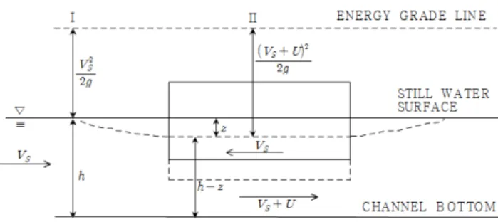
The complicated variations of vessel’s resistance and squat occurs in a restricted waterway because of a lateral and vertical limitation of the waterway. Schijf(1949) developed a method based on preservation of energy to compute the limiting speed. This speed is the maximum possible sailing speed which self propelled vessels cannot exceed for a certain vessel in a restricted waterway of given dimensions.
The following equation is obtained from the Bernoulli theorem applying for the cross-sections Ⅰ and Ⅱ in Figs.
1 and 2.
Fig. 1 Longitudinal section of channel
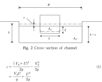
Fig. 2 Cross-section of channel
(1)
where, depicts the maximum water-level depression(or squat) at amidships section, the vessel's service speed,
the maximum return current velocity along a vessel at amidships section, the gravitational acceleration.
Applying the continuity condition for the two cross sections Ⅰ and Ⅱ, the following equation is obtained.
(2)
where, describes the water discharge, the channel cross section, the midship cross section of a vessel and
the waterway’s breadth at water-level. Combining the equation (1) with (2), the equation (3) can be easily obtained.
(3)where, BR(== : demonstrates the vessel's breadth, the vessel's draft and (=) the area average water depth) is the blockage ratio which is sometimes used in combination of the depth draft ratio () with the non-dimensional width(b/B). (= ) the depth Froude number.
And in addition the following equation on the return current velocity is derived from the equations (1) and (2).
(4)
where, (= ) demonstrates the Froude number
with the return current. The Froude number with the return current and the dimensionless squat / are a function of the depth Froude number and the blockage ratio BR. In cases and BR are large, the cross section beside the hull is insufficient to discharge the return current and an excess of water is piled up in front of the vessel. In case of insufficient clearance under the keel, the vessel will hit the sea bottom due to the squat.
When a correction factor proposed by Groenveld(1999) is applied to the equation (1), the following equation is obtained.
(5)
where, (=1.4-0.4lim) means a correction factor for the non-uniform distribution of the return current . The symbol lim shows the vessel's maximum service speed and self propelled vessels cannot exceed it as will be stated later. The factor varies from 1.05(lim=0.875) to 1.2 (lim=0.5).
Applying the equation (5) for the equation (3) and (4) respectively, the equations regarding and including
are newly derived as follows.
(6)
(7)
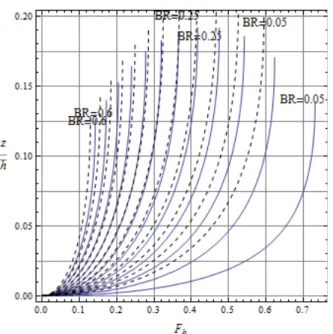
Fig. 3 represents the relationship between the Froude number and the non-dimensional squat for various values(0.05-0.6 : 0.05 intervals) of the blockage ratio BR. In the Fig. 3 the solid lines and the dotted lines respectively represent values for the cases that =1.0 and =1.2.
For a given BR, has a certain maximum value beyond which it is impossible for the vessel to proceed. If there is insufficient clearance under the keel, the vessel will strike the canal bottom before this maximum speed is attained. A value of will be evaluated for an arbitrary
. In the case of =1.2, the squat has a little greater value than that of =1.0.
Fig. 3 Relationship between and for various values of BR(solid lines : =1.0, dotted lines : =1.2)
Fig. 4 represents the relationship between and for various values(0.05-0.6 : 0.05 intervals) of the blockage ratio BR In the Fig. 4, the solid lines and the dotted lines respectively represent values for the cases that =1.0 and
=1.2.
For a given BR, has a certain maximum value beyond which it is impossible for the vessel to proceed. A value of will be evaluated for an arbitrary such as the squat in Fig. 3. In the case of α=1.2, has a greater value than that of =1.0.
Fig. 4 Relationship between and for various values of BR(solid lines : =1.0, dotted lines : =1.2)
The maximum discharge max can be derived from the continuity equation (2).
maxlim
lim
(8)
Substituting the equation (1) with lim instead of into the equation (8), the following equation is obtained.
max lim (9)
Differentiating the equation (9), and setting the result to zero, the resulting relation is derived.
max
lim
lim
(10)
Applying the equation (10) for the equation (3), the equation (11) can be obtained. For a given BR, lim gives the maximum value beyond which it is impossible for the vessel to proceed.
lim
lim
(11)
where, lim(lim ) depicts the Froude number with lim.
In cases of extremes of BR(=0, 1), the followings hold:
lim lim when (12a)
lim lim when (12b)
At an unrestricted waterway a vessel is able to sail at a maximum speed equal to the wave speed in shallow water.
BR from 0.1 to 0.3 is mostly applied for inland waterways.
The following equation is derived from the equation (10)
lim
lim (13)
And in addition, the following equation on the Froude number with the maximum return current velocity
lim is obtained.
lim
lim (14)
where, (=lim )is the Froude number with
lim.
Applying the equation (5) for the equation (13) and (14) respectively, the equations regarding lim and
including are derived.
lim
lim
(15)
lim lim
lim
lim (16)
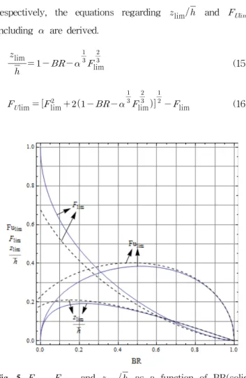
Fig. 5 lim, and lim as a function of BR(solid lines : =1.0, dotted lines : =1.2)
Fig. 5 shows the extremes such as lim, and
lim with the variations of the blockage ratio BR. The effect of is greater in cases that the blockage ratio BR is smaller.
In the case of Ara waterway which is BR=0.142, /d=1.4,
lim, and lim respectively is 0.554, 0.268 and 0.184 for =1.0 . Therefore, the ship's maximum service speed
lim results in 8.4(knots) and self propelled ships cannot exceed it.
3. Model experiments
In shallow or restricted waters, taking the characteristics of the shipwaves generated by a moving ship into consideration, the maximum dimensionless wave height
max which is a kind of the secondary wave system, is
mainly governed by the following parameters.
max
(17)where, is the perpendicular distance from the sailing line. It is simply shown that the maximum dimensionless wave height is the functions of the depth Froude number which is mainly dependent on the velocity of the vessel with respect to the water depth, the non-dimensional water depth, the non-dimensional width and the non-dimensional distance. A series of model experiments were carried out in the model basin (28m in length, 6m in width and 1m in depth) of the Navigational Operating Laboratory at Korea Maritime University. Fig. 6 shows the sketch of a shipwave experiment.
Fig. 6 Sketch of shipwave experiment
In these experiments, a ship model was towed at various speeds(0.20-1.01m/s) in water of a constant depth, and the wave profiles were measured with capacitance-type wave gauges at various distances along a perpendicular to the sailing line after the model ship had attained a constant speed. The model canal and the model ship respectively had the scale of 1: 60 for the Ara waterway and an R/S(River/Sea) ship under consideration in the canal was chosen as a model ship. The dimensions of the model canal and ship used in experiments are demonstrated in Table 1.
Table. 1 Dimensions of model canal and ship Unit:m
Type Breadth
(B, b)
Depth(h) or
Draft (d) Length Rectangular
Canal 1.333 0.105
River/Sea
Container ship 0.265 0.075 2.0
A typical example of a wave height record is shown in Fig. 7. The maximum wave height represents the vertical distance where the distance from a crest to a trough is largest. If a ship speed or its blockage ratio is large sufficiently, the excess water which does not pass because of insufficient clearance around the ship must be dammed up in front of the ship in the form of a surge or bore ahead and negative disturbance aft of the ship. As soon as the ship passes, the water-level goes down and rises again.
Fig. 7 Example of waveform
4. Experimental results
Fig. 8 shows the maximum non-dimensional wave height for the case of BR=0.142. The observation locations(S/b) are 1.0 and 2.0. The maximum wave height is nearly constant without regard to the distance S in a restricted water. It seems that the almost same high sized wave heights take place on the whole waterway in a restricted water because of the partial standing waves with incident and reflected waves. For the case that corresponds to 0.554, the maximum dimensionless wave height is beyond 0.2 which is a considerably large value(refer to Table 2).
Fig. 8 Maximum dimensionless wave heights as a function of (BR=0.142)
Table 2 Maximum dimensionless wave heights as a function of (BR=0.142, S/b=1)
0.2 0.3 0.4 0.5 0.554
max 0.058 0.082 0.113 0.132 0.214
0.7 0.8 0.9 1.0
max 0.473 0.869 1.046 1.256
Fig. 9 denotes the dimensionless wave heights on three types of waterways. In the Fig., “One side opened” means that one side has a bank but the other side does no bank(endless). In one-side opened channel, the observation locations are in between the bank and the ship.
Dimensionless water heights of restricted waterway and one-side opened waterway are respectively 2 and 1.5 times larger than those of shallow waterway.
Fig. 9 Dimensionless wave heights of three types of waterways( /d=1.4)
Fig. 10 shows the effect of b/B on the dimensionless height with a parameter S/b. For the case of relatively nar- row channel, the wave heights are considerably large on the whole waterway. On the contrary, for the case of wider
Fig. 10 Effect of b/B on wave heights( , /d=1.4)
channel, the wave heights are smaller and decrease with an increase of the ship’s distance. Consequently, under 0.2 of b/B, the wave heights is lower than 20% of the draft.
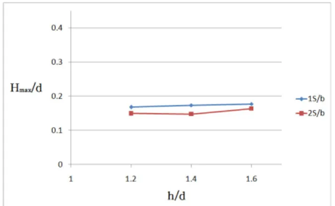
Fig. 11 shows the characteristics of max as a function of the water depth. The wave heights are almost constant with water depth increase. It means that the effect of non-dimensional water depth on the heights is negligibly little.
Fig. 11 Effect of /d on wave heights( , b/B=0.2)
4. Conclusions
Main conclusions obtained in the present study are summarized as follows.
y and / with a correction factor can be newly evaluated for an arbitrary depth Froude number and they are a function of the depth Froude number and the blockage ratio BR.
y The maximum service speed lim of a scheduled vessel in Ara waterway is 8.4 knots and the vessel cannot exceed it.
y The almost same high-sized wave heights take place on the whole waterway in a restricted water without regard to the distance from the sailing line.
y The wave heights in a restricted waterway such as the case of Ara waterway exceed 20% of ship's draft.
y Dimensionless water heights in a restricted waterway is 2 times larger than that in a shallow waterway.
y The effect of the non-dimensional width b/B on the wave height is much larger than that of non-dimensional water depth /d.
Acknowledgements
This research was supported by the Korea Sanhak
Foundation in 2009. The author would like to express his gratitude for the financial assistance provided by the Korea Sanhak Foundation.
References
[1] Gang, S. J., Kim, M. G., and Kim, C. J,(2009), "A Study on Shape and Height of Shipwaves", Journal of Korean Navigation and Port Research, Vol. 33, No. 2, pp.
105-110.
[2] Gang, S. J., Kim, S. K., Son, C. B., Kim, J. S., Hong, J.
H., and Kim, C. J. (2007), “A study on the characteristics of shipwaves”, Journal of Korean Navigation and Port Research, Vol. 31, No. 5, pp.
339-344
[3] Groenveld, R.(1999), "Service systems in ports and inland waterways", TUDelft lecture notes.
[4] Johnson, J. W.(1958), “Ship waves in navigation channel”, Proc. Conf. Coastal Eng., 6Th, Miami Beach, Fla. pp. 666-690.
[5] Norrbin, N. H.(1986), "Fairway Design with Respect to Ship Dynamics and Operational Requirements", SSPA Research Report No. 102, SSPA Maritime Consulting, Gothenburg, Sweden.
[6] Schijf, J. B.(1949), "Protection of Enbankments and Bed in Inland and Maritime Waters, and in Overflow or Weirs", XVII international Navigation Congress, Lisbon, Section I, pp. 61-78.
[7] Taylor D. W.(1943), "The Speed and Power of Ships", U. S. Govt. Printing Office.
[8] US Army Corps of Engineers(2006), "Hydraulic Design of Deep-Draft Navigation Projects"
Received 9 August 2011 Revised 8 September 2011 Accepted 9 September 2011