https://doi.org/10.7848/ksgpc.2019.37.2.71
Geolocation Error Analysis of KOMPSAT-5 SAR Imagery Using Monte-Carlo Simulation Method
Choi, Yoon Jo 1)·Hong, Seung Hwan 2)·Sohn, Hong Gyoo 3)
Abstract
Geolocation accuracy is one of the important factors in utilizing all weather available SAR satellite imagery.
In this study, an error budget analysis was performed on key variables affecting on geolocation accuracy by generating KOMPSAT-5 simulation data. To perform the analysis, a Range-Doppler model was applied as a geometric model of the SAR imagery. The results show that the geolocation errors in satellite position and velocity are linearly related to the biases in the azimuth and range direction. With 0.03cm/s satellite velocity biases, the simulated errors were up to 0.054 pixels and 0.0047 pixels in the azimuth and range direction, and it implies that the geolocation accuracy is sensitive in the azimuth direction. Moreover, while the clock drift causes a geolocation error in the azimuth direction, a signal delay causes in the range direction. Monte-Carlo simulation analysis was performed to analyze the influence of multiple geometric error sources, and the simulated error was up to 3.02 pixels in the azimuth direction.
Keywords : KOMPSAT-5, SAR, Geolocation Error, Sensitivity Analysis, Monte-Carlo Simulation
Original article
1. Introduction
The geometric model of the SAR imaging system can be defined by the Range-Doppler equations (Curlander, 1984;
Curlander and McDonough, 1991; Schreier, 1993). The geometric characteristics of the SAR (Specific Absorption Rate) imagery shows a different pattern from that of the typical optical imagery defined by the collinearity equation, which makes it difficult to interpret the geolocation accuracy of the images. For optical imaging system, the position and attitude of the satellites and IOPs (Interior Orientation Parameters) of the sensors play an important role in geolocation accuracy, whereas the satellite position and velocity, clock drift, signal delay and atmospheric condition are important variables for the SAR imaging system that generate the imagery through the radar signal processing (Frey et al., 2004; Toutin, 2004;
Schwerdt et al., 2010; Hong et al., 2013).
Obviously, accurate satellite orbits, sensors, and atmospheric condition information can ensure high geometric accuracy of the SAR imagery (Eineder et al., 2011; Schubert et al., 2012). However, for utilizing real-time satellite imagery, it is difficult to obtain accurate information about SAR imaging geometry and can vary depending on the shooting time and place (Toutin, 2004; Schubert et al., 2010). For this reason, geometric correction techniques based on GCPs (Ground Control Points) have still used as an alternative for practical applications. However, when observing non-accessible areas where GCP surveying is not practically easy, the analysis of the geolocation accuracy of the images should be preceded in order to effectively utilize the SAR images in urgent situations such as disaster.
For the TerraSAR-X system of Germany, rigorous analysis
Received 2019. 03. 17, Revised 2019. 04. 11, Accepted 2019. 04. 29
1) Member, School of Civil and Environmental Engineering, Yonsei University (E-mail: [email protected]) 2) Member, Stryx Inc. (E-mail: [email protected])
3) Corresponding Author, Member, School of Civil and Environmental Engineering, Yonsei University (E-mail: [email protected])
This is an Open Access article distributed under the terms of the Creative Commons Attribution Non-Commercial License (http://
and calibrations of geolocation accuracy were performed after the launch in 2007. The shift in the azimuth direction of the system and internal electronic delay of the sensor were considered as major variables for geometric correction and monitored using corner reflectors (Döring et al., 2007;
Schwerdt et al., 2007; Schubert et al., 2010). Yoon et al. (2009) analyzed that the geolocation accuracy can be achieved up to 20cm by using the orbit information provided by the POD (Precision Orbit Determination) for TerraSAR-X. Schubert et al. (2012) analyzed the effects of signal delay and Earth’s motion by modeling each variable, and Eineder et al. (2011) demonstrated that Earth surface displacements can be measured at a centimeter level. By monitoring and calibrating the error sources, the TerraSAR-X is able to achieve more than 2m accuracy (Nonaka et al., 2008; Schwerdt et al., 2008a; Schwerdt et al., 2008b).
Corner reflectors for KOMPSAT-5 were also installed for geometric and radiometric calibration before the mission was launched, and simulation tests were performed to estimate the orbit accuracy (Hwang et al., 2011; Yoon et al., 2011). Jung et al. (2014) analyzed that orbit precision can be obtained up to 12.77cm by using POD technique. Hong et al. (2013) conducted a simulation analysis to analyze the effects of geometric error factors in the project for the preparation of KOMPSAT-5 and KOMPSAT-6. The sensitivity analysis was performed using virtual dataset based on parameters of TerraSAR-X system which has similar specification with KOMPSAT-5. However, no study has been analyzed the factors causing geometric errors using KOMPSAT-5 imagery.
Therefore, the purpose of this study is to analyze geometric error factors of KOMPSAT-5 satellite. First of all, simulated dataset was generated from information about the satellite orbit and sensor and relationship between the image coordinate and the ground coordinate of the target, and then error budget analysis was performed on critical parameters.
The accuracy of KOMPSAT-5 SAR imagery was verified using GCPs extracted from the orthorectified image and the airborne LiDAR (light Detection and Ranging) DSM (Digital Surface Model). Then, the influence of critical variables was analyzed by assigning a simulated biases to the header
Monte-Carlo simulation analysis was performed to analyze the combined effects of the critical variables.
2. Methods
2.1 Main geometric error sources of SAR sensors Generally, the geometry of SAR imaging system is defined by the Range-Doppler model. In this geometric relationship, satellite orbit and sensor information play an important role in geolocation accuracy (Toutin, 2004; Schwerdt et al., 2010).
In the past, due to the low precision of the SAR satellite orbit information, models which calibrate satellite position and velocity information was primarily used (Toutin, 2004).
However, recent studies have been conducted to analyze the stability of the SAR sensor and the effect of geodynamic implications, since centimeter-level geolocation accuracy can be ensured by applying POD technology using dual frequency GPS (Global Positioning System) (Hong et al., 2017).
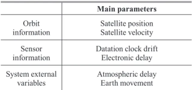
Hong et al. (2013) divided the critical variables affecting a geometric geolocation accuracy into three main geometric parameters according to the SAR sensor geometry model.
Three main geometric parameters contain platform orbital information, sensor information, and system external variables. The geometric error factors in the SAR imaging system are shown in Table 1. Each factor will be briefly discussed in the following sections.
Table 1. Main geometric parameters in SAR imaging system Main parameters
Orbit
information Satellite position Satellite velocity Sensor
information Datation clock drift Electronic delay System external
variables Atmospheric delay
Earth movement
2.1.1 Satellite orbit information
In the past, many low-orbit satellites were equipped with a single frequency GPS receiver due to cost aspects and techni- cal problems, and platform orbit information had a position-
al error of hundreds of meters. Thus, geometric correction models was developed by focusing on the orbit calibration of the SAR satellite imaging system. However, recently launched satellites such as TerraSAR-X and KOMPSAT-5 equipped with dual frequency GPS receivers which can be used for POD technique. Ionosphere errors can be accurately eliminated by utilizing POD technique, and it provide cen- timeter-level orbit accuracy (Jung et al., 2014; Hong et al., 2017).
2.1.2 Satellite sensor information
If the accuracy of the orbit information is guaranteed, the error in the sensor information significantly affects the pixel allocation accuracy of the SAR imagery (Curlander and McDonough, 1991). The time difference between the satellite orbit information and the radar system causes a shift in the azimuth direction of the imagery in proportion to the PRF (Pulse Repetition Frequency) (Breit et al., 2010;
Hong et al., 2017; Eineder et al., 2001). As satellite velocity increases, calculated distances between satellite and targets are distorted and eventually clock biases cause the shift in the range direction (Curlander and McDonough, 1991).
The electronic delay of the signal occurs in the process of estimating the signal propagation time through radar echo sampling. The signal delay has a direct effect on measuring the range distance between the SAR sensor and the observed target, and this causes image coordinate errors mainly in the range direction (Hong et al., 2017; Eineder et al., 2011).
2.1.3 System external variables
If the accuracy of the orbit and sensor information is ensured, the effects of atmospheric delay and Earth movement can be measured directly. Eineder et al. (2011) reported that the changes in the solid Earth tides and tropospheric water vapor cause a large error in the range direction, and Jehle et al. (2008) stated that the influences of the atmosphere in the high-resolution SAR systems play an important role in geolocation accuracy and are an essential consideration.
The radar echo time in the atmosphere is slower than in the vacuum because of refraction which occurs in the atmosphere, and this causes an overestimated range distance
when the light speed in the vacuum is used to derive the range distance (Breit et al., 2010; Schubert et al., 2012). The error of the range distance due to the path delay is approximately 2~4m and depends on the atmospheric conditions and length of the path (Ager and Bresnahan, 2009).
The periodic fluctuations of the Earth occur vertically up to 40cm in the mid-latitude (Schubert et al., 2012). While the Earth’s vertical variations cause a maximum SAR biases of 15cm compared to the state without tidal phenomena, they result in very small horizontal displacements of several centimeters in the azimuth direction (Schubert et al., 2012).
The errors caused by Earth movement are negligible in the application of SAR imagery because they are only 10~20cm (Melchior, 1974; Milbert, 2016; Penna et al., 2008).
2.2 Generation of simulation data
In the SAR imaging system, the relationship between the image coordinates and the target located on the ground can be defined as the Range and Doppler equations. The Range and Doppler equations can be represented by Eqs. (1) and (2), respectively (Curlander and McDonough, 1991).
(1)
∙
(2)where, and are the position vector of the SAR sensor and ground target, and and are the velocity vector of the SAR sensor and ground target. The position and velocity of the satellite continuously change while the images are acquired, and due to these characteristics, the satellite orbit model can be defined as a time-dependent polynomial equation. The position of the satellite can be defined as a second order time-dependent equation, and the satellite velocity is defined as the time derivative of the satellite position vector. The satellite position and velocity equations are as follows Eqs. (3) and (4).
(3)
(4)
where, are the satellite position parameters, and
and
are the biases given for a sensitivity analysis on the satellite orbital position and velocity, respectively.
Assuming that the images are processed with zero Dop- pler, the Doppler equation can be represented as Eq. (5). The imaging time for the target ground coordinates can be calcu- lated by applying the Newton-Raphson method (Hong et al., 2013). The pixel sampling time () can be calculated through iterative calculation until the difference between and
from Eq. (6) converges below a certain value.
∙ (5) (6)
′
Using the pixel sampling time (), The azimuth pixel coordinates () can be calculated from Eq. (7) and the range pixel coordinates ( ) can be calculated by Eq. (8).
(7)
(8)
×
where, is the imaging start time, is the pulse repetition frequency, and is the range sampling frequency. is the distance from the column direction to the first pixel, is the range distance between the satellite and the target, and is the speed of the light. In order to analyze the position accuracy according to the precision of sensor information, a bias () was assigned to the satellite orbit time to generate error simulation data according to the signal sampling precision, and a bias () was given to the signal propagation time in the range distance to generate the error simulation data according to the electronic time delay.
2.3 Monte-Carlo simulation
simulation techniques that predict uncertainty and use a probabilistic approach to solve problems by simulating all possible scenarios. Monte-Carlo simulation methods have been applied in many cases such as performing the uncer- tainty analyses of geolocation accuracy caused by various error sources (Bresnahan and Jamison, 2007; Zanin, 2014).
Monte-Carlo simulation is a method to obtain an approxi- mate solution of a problem by repeatedly performing sim- ulations using randomly extracted numbers. The process of the simulation is consisted of 1) selection of uncertain input variables, 2) determination of probability distribution re- flecting population parameter of input variables, 3) method selection and implementation, and 4) results analysis (Kim et al., 2012).
In this study, the error budget analysis flow is as shown in Fig. 1. First, a metadata is read from the SAR data, and then the precisions for the main geometric error factors are set.
This can be used to generate simulation data and geolocation errors can be estimated through performing simulation based on the physical sensor model.
Fig. 1. Error budget analysis flow based on Monte-Carlo simulation
3. Results
3.1 KOMPSAT-5 imagery
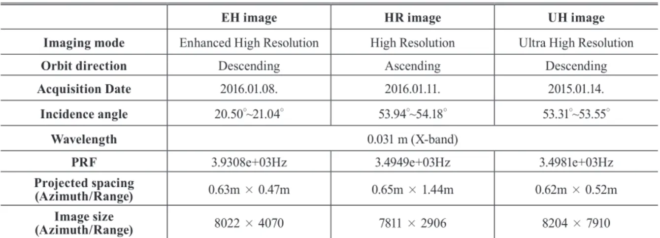
In this study, the analysis was performed using KOMPSAT-5 satellite images equipped with X-band SAR sensor launched for the first time in Korea. The images were taken in EH (Enhanced High resolution), HR (High Resolution) and UH (Ultra High resolution) modes. The altitude of the study area is about 50~1,250m, and it covers various types of land cover such as mountain, urban, rural, bare soil, and water. Table 2 shows the basic information of
3.2 Geolocation accuracy of KOMPSAT-5 imagery
In order to confirm the geolocation accuracy of the actual KOMPSAT-5 images, 43 GCPs were extracted from KOMPSAT-5 images, the orthorectified image of 50cm resolution, and DSM data produced by airborne LiDAR.
Satellite orbits were modeled using satellite position and velocity information, and image coordinates were determined from satellite sensor information and ground coordinates.
SAR images used in the analysis and distribution of GCPs can be shown as Fig. 2.
5001000150020002500300035004000 1000
2000 3000 4000 5000 6000 7000
8000 -20
-10 0 10 20 30 40 50 Control points 60
500 1000 1500 2000 2500
1000 2000 3000 4000 5000 6000 7000
-20 -10 0 10 20 30 40 50 Control points 60
10002000 300040005000 60007000 1000
2000 3000 4000 5000 6000 7000
8000 -20
-10 0 10 20 30 40 50 Control points 60
(a) EH image (b) HR image (c) UH image Fig. 2. KOMPSAT-5 SAR images and distribution of GCPs
As a result of the KOMPSAT-5 geolocation accuracy analysis, the errors were 1.58 pixels in the row direction and –3.60 pixels in the column direction in the EH mode image.
In the HR mode image, -1.67 pixels in the row direction and 5.21 pixels in the column direction. And in the UH mode image, there is an error of –0.45 pixels in the row direction and –17.52 pixels in the column direction. Therefore, the
average RMSEs (Root Mean Square Errors) of geolocation accuracy of each image were 3.99 pixels in EH image, 5.51 pixels in HR image, and 17.54 pixels in UH image. However the standard deviations of each image were 1.00 pixel, 1.07 pixels, and 0.85 pixels, respectively. The errors mainly appeared in the column direction.
These patterns came from a complex effect of error factors such as the altitude information and accuracy of the ground coordinates, the atmospheric delay, and the electronic time delay of the SAR sensor. When the GCPs are extracted from the high resolution images, the errors in the orthorectified image and the digital map are also included in the positional error (Hong et al., 2013). Fig. 1 is the geolocation accuracy of GCPs in the images, the horizontal axis indicates the error in the row direction, and the vertical axis indicates the error in the column direction.
-20 -15 -10 -5 0 5 10 15 20
Row (Pixel) -20
-15 -10 -5 0 5 10 15 20
Column (Pixel)
EH HR UH
Fig. 3. Geolocation accuracy of KOMPSA T-5 images in the study area
EH image HR image UH image
Imaging mode Enhanced High Resolution High Resolution Ultra High Resolution
Orbit direction Descending Ascending Descending
Acquisition Date 2016.01.08. 2016.01.11. 2015.01.14.
Incidence angle 20.50°~21.04° 53.94°~54.18° 53.31°~53.55°
Wavelength 0.031 m (X-band)
PRF 3.9308e+03Hz 3.4949e+03Hz 3.4981e+03Hz
Projected spacing
(Azimuth/Range) 0.63m × 0.47m 0.65m × 1.44m 0.62m × 0.52m
Image size
(Azimuth/Range) 8022 × 4070 7811 × 2906 8204 × 7910
Table 2. Information of KOMPSAT-5 images used for the study
Journal of the Korean Society of Surveying, Geodesy, Photogrammetry and Cartography, Vol. 37, No. 2, 71-79, 2019
Fig. 4 shows 50 times magnified error sizes between points calculated by physical sensor model and GCPs. Even though the error sizes are different, the error patterns of similar tendencies are shown in all three images used in the analysis.
500 10001500 20002500 3000 35004000 1000
2000 3000 4000 5000 6000 7000 8000
Control point Error (X50)
500 1000 1500 2000 2500
1000 2000 3000 4000 5000 6000
7000 Control point
Error (X50)
1000 2000 3000 40005000 6000 7000 1000
2000 3000 4000 5000 6000 7000
8000 Control point
Error (X50)
(a) EH image (b) HR image (c) UH image Fig. 4. Distribution of the geolocation error
3.3 Sensitivity analysis by geometric error sources
Satellite position and velocity biases, electronic delays, atmospheric delays, and clock drift are main variables that cause geolocation errors in SAR imaging system. In order to analyze the effect of geometric error in the imaging system, simulation analysis was performed by giving simulated biases to the orbit and sensor information. In this case, it is assumed that there is no error in other variables besides the variables given the simulated biases. Figs. 5 and 6 are simulation results for errors in satellite orbit information. Fig.
5 shows the simulation errors by the satellite position biases, and the relationship between the errors and biases in both the azimuth and range direction is analyzed to be linear. Hwang et al. (2011) reported that the orbit accuracy of KOMPSAT-5 is less than 20cm, and when the position biases of 20cm in X, Y and Z direction of orbit information occur, the maximum errors are 0.26 pixels in the azimuth direction and 0.37 pixels in the range direction.
(a) Azimuth direction (b) Range direction Fig. 5. Simulated error by satellite position bias
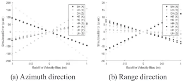
Fig. 6 is the result of analyzing the errors by the satellite velocity biases. The relationship between the errors and biases in both the azimuth and range direction is also analyzed to be linear. Hwang et al. (2011) reported that the velocity information of KOMPSAT-5 provided by POD technique is guaranteed to 0.03cm/s. When velocity bias of 0.03 cm/s occurs in the azimuth and range direction, the maximum errors are 0.054 pixels and 0.0047 pixels respectively.
Since the satellite velocity information significantly affects the determination of the pixel sampling time based on the Doppler equation, biases of satellite velocity information have considerable influence on the error occurring in the azimuth direction. On the other hand, in the range direction, as the image coordinates are determined by the distance between the sensor and the ground target, the satellite velocity accuracy is relatively less affected.
(a) Azimuth direction (b) Range direction Fig. 6. Simulated error by satellite velocity bias
When the position of the satellite is estimated based on the POD method, the accuracy of the sensor information such as the clock drift and the electronic delay of the signal might mainly affect the geolocation accuracy. Figs. 7 and 8 show the simulation results for the error sources included in the sensor information. As shown in Figs. 7 and 8, the clock drift and the electronic delay of the signal have a linear correlation with respect to the pixel allocation error in the azimuth and range direction, respectively. There is little influence on the clock drift in the range direction and the electronic delay of the signal in the azimuth direction. This result implies that the clock drift and electronic delay directly affect the pixel allocation error in the azimuth and range direction, respectively.
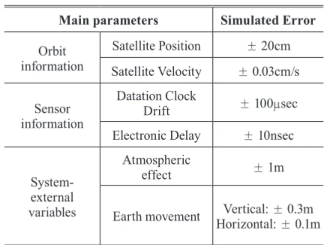
Table 3. Simulated biases for error budget analysis Main parameters Simulated Error Orbit
information
Satellite Position ± 20cm Satellite Velocity ± 0.03cm/s Sensor
information
Datation Clock
Drift ± 100μsec
Electronic Delay ± 10nsec
System- external variables
Atmospheric
effect ± 1m
Earth movement Vertical: ± 0.3m Horizontal: ± 0.1m
In order to perform the Monte-Carlo simulation, 100,000 virtual points with random error are applied. For generating simulation data, 68%, 90%, 95%, and 99% confidence level were applied, and simulation data is generated randomly within a set confidence interval. The Monte-Carlo simulation results are shown in Table 4.
As a result of Monte-Carlo simulation, the simulated biases cause ±1.11~3.02 pixels in the azimuth direction and
±0.37~2.92 pixels in the range direction depending on the confidence levels. It is analyzed that the errors in the azimuth direction were greater than the errors in the range direction.
This result can be explained by the fact that the bias of satellite velocity is sensitive to the geolocation accuracy in the azimuth direction from the results analyzed earlier.
As the width of the confidence interval increases, the estimated errors in the images are increased. However, the errors are up to 3.02 pixels at the 99% confidence level, which can make it feasible to correct precisely using (a) Azimuth direction (b) Range direction
Fig. 7. Simulated error by clock drift bias
(a) Azimuth direction (b) Range direction Fig. 8. Simulated error by signal delay bias
3.4 Analysis of error simulation for complex variables
Each of the above-mentioned error sources operates in a complex manner, which affects the geolocation accuracy of the imagery. A Monte-Carlo simulation technique was performed to calculate the error budget induced by the simulated biases on the main error sources.
In order to analyze the effect of error factors on the geolocation accuracy of satellite images, the simulation value of each error source is set in considering the study results of Hwang et al. (2011) and Hong et al. (2013) (Table 3).
Confidence level
EH image HR image UH image
Azimuth Range Azimuth Range Azimuth Range
68% 1.1480 1.1368 1.1097 0.3733 1.1683 1.0324
90% 1.8989 1.8746 1.8366 0.6171 1.9293 1.7141
95% 2.2543 2.2233 2.1759 0.7316 2.2942 2.0268
99% 2.9714 2.9235 2.8672 0.9640 3.0155 2.6656
Table 4. Monte-Carlo simulation results (unit: pixel)
geometric correction model since the distribution of errors has systematic patterns.
4. Conclusion
In this study, the effects of main geometric error sources on geolocation accuracy were analyzed through the sensitivity analysis of each error source and complex variables to KOMPSAT-5 which is Korea’s first high resolution SAR satellite. By performing Monte-Carlo simulation, 100,000 virtual points with random error the following results are obtained.
First, the errors in satellite orbital position and velocity showed a linear relationship with the geolocation error in both the azimuth and range direction. In addition, satellite velocity errors are analyzed to be sensitive to geolocation accuracy in the azimuth direction.
Second, the clock drift has a linear relation with the geolocation error in the azimuth direction. On the other hand, the electronic and atmospheric signal delay have a linear relation with the geolocation error in the range direction.
Third, as a result of the analysis on the Monte-Carlo simulation, the expected errors recorded in existing researches can cause 0.98~2.97 pixels error. Using the GCPs, the actual geolocation accuracy of high-resolution KOMPSAT-5 SAR imagery was –19.50~7.68 pixels. It was because the accuracy of the orbit information was not stable and calibrated. To ensure the geolocation quality of the SAR imagery, the orbit information must be controlled by periodical calibration with other information such as signal delay and datation clock drift. The 0.37~3.02 pixels standard deviations of the geolocation accuracy checked by the GCPs demonstrated that the systematic errors have the linear relationship with the geolocation on a whole image and can be corrected by the geometric calibration process for the error sources.
By this research, it is proved that the geolocation accuracy can be controlled by monitoring and correcting the error sources. Moreover, the results demonstrated that the geometric correction for the parameterized error sources can correct the sub-pixel geolocation accuracy. The analysis results can be contributed for the practical application of
fusion and radargrammetry which require high geolocation accuracy.
Acknowledgement
This work was supported by DAPA(Defense Acquisition Program Administration) and ADD(Agency for Defense Development).
References
Ager, T.P. and Bresnahan, P.C. (2009), Geometric Precision in Space Radar Imaging: Results from TerraSAR-X, NGA CCAP Report.
Breit, H., Fritz, T., Balss, U., Lachaise, M., Niedermeier, A., and Vonavka, M. (2010), TerraSAR-X SAR processing and products, IEEE Transactions on Geoscience and Remote Sensing, Vol. 48, No. 2, pp. 727-740.
Bresnahan, P.C. and Jamison, T.A. (2007), A Monte Carlo simulation of the impact of sample size and percentile method implementation on imagery geolocation accuracy assessments. In Proceedings of ASPRS 2007 Conference, 7-11 May, Tampa, Florida, USA, pp. 7-11.
Curlander, J.C. (1984), Utilization of spaceborne SAR data for mapping, IEEE Transactions on Geoscience and Remote Sensing, 2, pp. 106-112.
Curlander, J.C. and McDonough, R.N. (1991), Synthetic Aperture Radar: Systems and Signal Processing, New York, USA, John Wiley & Sons, INC.
Eineder, M., Breit, H., Adam, N., Holzner, J., Suchandt, S., and Rabus, B. (2001), SRTM X-SAR calibrations results, IEEE Geoscience and Remote Sensing Symposium, 9–13 July, Sydney, Ausralia, pp. 748-750.
Eineder, M., Minet, C., Steigenberger, P., Cong, X., and Fritz, T. (2011), Imagine geodesy – toward centimeter- level ranging accuracy with TerraSAR-X, Geoscience and Remote Sensing, IEEE Transactions on Geoscience and Remote Sensing, Vol. 49, No. 2, pp. 661-671.
Frey, O., Meier, E., Nüesch, D., and Roth, A. (2004), Geometric error budget for TerraSAR-X, Proceedings of the 5th European Conference on Synthetic Aperture Radar
Hong, S., Choi, Y., Park, I., and Sohn, H.G. (2017), Comparison of orbit-based and time-offset-based geometric correction models for SAR satellite imagery based on error simulation, Sensors, 17, 170.
Hong, S.H., Sohn, H.G., Kim, S.P., and Jang, H.S. (2013), Error budget analysis for geolocation accuracy of high resolution SAR satellite imagery, Journal of the Korean Society of Surveying, Geodesy, Photogrammetry and Cartography, Vol. 31, No. 6-1, pp. 447-454. (in Korean with English abstract)
Hwang, Y., Lee, B.S., Kim, Y.R., Roh, K.M., Jung, O.C., and Kim, H. (2011), GPS-based orbit determination for KOMPSAT-5 satellite, ETRI Journal, 33, pp. 487-496.
Jehle, M., Perler, D., Small, D., Schubert, A., and Meier, E. (2008), Estimation of atmospheric path delays in TerraSAR-X data using models vs. measurements, Sensors, 8, pp. 8479-8491.
Jung, O., Chung, D., Kim, E., Yoon, J., and Hwang, Y. (2014), Analysis on the orbit accuracy of KOMPSAT-5, Aerospace Engineering and Technology, Vol. 13, No. 2, pp. 108-114.
Kim, Y.J., Park, C.S., and Kim, I.H. (2012), Sampling methods and stochastic inference in Monte Carlo building simulation, Architectural Institute of Korea, Vol. 28, No.
6, pp. 227-236. (in Korean with English abstract)
Melchior, P. (1974), Earth tides, Geophysical Surveys, Vol. 1, No. 3, pp. 275-303.
Milbert, D. (2016), Solid Earth Tide, http://geodesyworld.
github.io/SOFTS/solid.htm (last date accessed: 25 April 2019).
Nonaka, T., Ishizuka, Y., Yamane, N., Shibayama, T., Takagishi, S., and Sasagawa, T. (2008), Evaluation of the geometric accuracy of TerraSAR-X, International Archives of the Photogrammetry, Remote Sensing and Spatial Information Science, 37, pp. 135-140.
Penna, N.T., Bos, M.S., Baker, T.F., and Scherneck, H.G.
(2008), Assessing the accuracy of predicted ocean tide loading displacement values, Journal of Geodesy, Vol. 82, No. 12, pp. 893-907.
Schreier, G. (1993), SAR Geocoding: Data and Systems, Karlsruhe, Germany, Wichmann.
Schubert, A., Jehle, M., Small, D., and Meier, E. (2010), Influence of atmospheric path delay on the absolute
geolocation accuracy of TerraSAR-X high-resolution products, IEEE Transactions on Geoscience and Remote Sensing, Vol. 48, No. 2, pp. 751-758.
Schubert, A., Jehle, M., Small, D., and Meier, E. (2012), Mitigation of atmospheric perturbations and solid earth movements in a TerraSAR-X time-series, Journal of Geodesy, Vol. 86, No. 4, pp. 257-270.
Schwerdt, M., Brautigam, B., Bachmann, M., and Döring, B.
(2008a), TerraSAR-X calibration results, In 7th European Conference on Synthetic Aperture Radar. VDE, pp. 1-4.
Schwerdt, M., Bräutigam, B., Bachmann, M., Doring, B., Schrank, D., and Gonzalez, J.H. (2008b), Final results of the efficient TerraSAR-X calibration method, In 2008 IEEE Radar Conference, 26-30 May, Rome, Italy, pp. 1-6.
Schwerdt, M., Brautigam, B., Bachmann, M., Doring, B., Schrank, D., and Gonzalez, J.H. (2010), Final TerraSAR-X calibration results based on novel efficient methods, IEEE Transactions on Geoscience and Remote Sensing, Vol. 48, No. 2, pp. 677-689.
Toutin, T. (2004), Geometric processing of remote sensing images: models, algorithm and methods, International Journal of Remote Sensing, Vol. 25, No. 10, pp. 1893-1924.
Yoon, J., Keum, J., Shin, J., Kim, J., Lee, S., Bauleo, A., Farina, C., Germani, C., Mappini, M., and Venturini, R.
(2011), KOMPSAT-5 SAR design and performance, 2011 3rd International Asia-Pacific Conference on Synthetic Aperture Radar (APSAR), 26-30 September, Seoul, Korea.
Yoon, Y.T., Eineder, M., Yague-Martinez, N., and Montenbruck, O. (2009), TerraSAR-X precise trajectory estimation and quality assessment, IEEE Transactions on Geoscience and Remote Sensing, Vol. 47, No. 6, pp. 1859- 1868.
Zanin, K.A. (2014), Quality analysis of image geolocation for a space synthetic aperture radar. Solar System Research, Vol. 48, No. 7, pp. 555-560.