in Laminated Composite Plates
Ahn, Jae-Seok* Woo, Kwang-Sung†
···
Abstract
The discrete-layer model is proposed to analyze the edge-effect problem of laminates under extension and flexure. Based on three-dimensional elasticity theory, the displacement fields of each layer in a laminate have been treated discretely in terms of three displacement components across the thickness. The displacement fields at bottom and top surfaces within a layer are approximated by two-dimensional shape functions. Then two surfaces are connected by one-dimensional high order shape functions. Thus the -convergent refinement on approximated one- and two-dimensional shape functions can be implemented independently of each other. The quality of present model is mostly determined by polynomial degrees of shape functions for given displacement fields.
For nodal modes with physical meaning, the linear Lagrangian polynomials are considered. Additional modes without physical meaning, which are created by increasing nodeless degrees of shape functions, are derived from integrals of Legendre polynomials which have an orthogonality property. Also, it is assumed that mapping functions are linear in the light of shape of laminated plates. The results obtained by this proposed model are compared with those available in literatures. Especially, three-dimensional out-of-plane stresses in the interior and near the free edges are evaluated and convergence performance of the present model is established with the stress results.
Keywords : -version of FEM; integrals of Legendre polynomials; laminate plate; free-edge stresses
···
†책임저자, 종신회원․영남대학교 건설시스템공학과 교수 Tel: 053-810-2593 ; Fax: 053-810-4622 E-mail: [email protected]
* 영남대학교 건설시스템공학과 박사후연구원
∙이 논문에 대한 토론을 2011년 2월 28일까지 본 학회에 보내주시 면 2011년 4월호에 그 결과를 게재하겠습니다.
1. Introduction
Over the past several decades, existence of high interlaminar stresses at the boundary-layer regions in the vicinity of the edge has been investigated using both approximate theoretical solutions and experi- mental observations. However, no exact solution is known to exist because of the inherent complexities involved in the problems. Among analytical methods, the first approximate solution for interlaminar shear stresses was proposed by Puppo et al. (1970). Rybicki (1971) proposed a three-dimensional finite element solution for quasi-three-dimensional problem. Pagano (1974) employed a higher-order displacement theory for estimation of transverse normal stress in axially loaded symmetric balanced laminates. Hsu et al.
(1977) proposed an improved quasi-three-dimensional
finite element method in order to determine the interlaminar stresses in symmetric balanced lamin- ates under uniform axial extension. Wang and Choi (1982a; 1982b) employed an approach based on Lekhnitskii’s complex variable potential to examine the free-edge stress singularities. Robbins et al.
(1996) present displacement based variable kinematic formulations with the assumption that the stresses and strains are dependent on all three coordinates.
Cho et al. (2000) used iterative method to analyze free-edge interlaminar stresses of composite laminates under extension, bending, twisting, and thermal loads. Recently, Nguyen et al. (2009) employed a multi-particle finite element for analysis of free-edge stresses of composite laminates subjected to mechanical and thermal loads.
Meanwhile, in the last few decades, several attempts
have been made to develop simple and efficient elements using displacement models satisfying only
-continuity requirements. Most implementations of the finite element methods are based on that the error of approximation is controlled by mesh refinement such that the size of the largest element mesh is reduced, fixing the polynomial degree of test and trial functions of elements, =1 or =2. On the other hand, mathematical justification showing the advantages of using a higher-order approximation of the field variables, so-called -version of FEM, was given by Babuska et al. (1981). Later on, the advantages of -version of FEM became quite obvious through not only experimental verification based on numerical analysis but also sound mathematical proof (Hong et al., 1996; Ghosh et al., 1998; Ahn et al., 2009, 2010;
Woo et al., 1989, 2003, 2007). Although automatic preprocessor is available for most commercially available application software packages, unfortunately, entirely automated mesh generators are still not available on markets. Thus, in this day and age, meshing work of preprocess is usually dependent on manpower of analysts. Thus, ideal meshing process would be fully performed by computers without human intervention. In the point of view of meshing work, usage of -version of FEM with coarse mesh and robustness, which performs well for a broad class of admissible input data, can be attractive.
In this study, discrete-layer model based on the -version of FEM is formulated to analyze the edge-effect problem of laminates under extension and flexure. Displacement fields of each layer in a laminate are treated discretely in terms of three displacement components across thickness. In modeling laminated plates, ply-by-ply representation across thickness is possible for resolving local stress and strain distribution. Thus, simple modeling can be obtained in analysis of the free-edge problems.
Also, quality of approximation of the present model is mostly determined by the polynomial degrees of shape functions for displacement fields. Sub-parametric concept is employed. Thus, approximate functions composed of linear Lagrangian polynomials and
integrals of Legendre polynomials are adopted for variation of displacements while mapping functions are linear by considering shape of laminated plates.
The results obtained with this finite element model are compared with those available in the literature.
Especially, three-dimensional out-of-plane stresses in the interior and near the free edges are evaluated and convergence performance of the present model is established with the stress results.
2. Hierarchical shape functions
From the theoretical point of view of general FEM, the quality of approximation is completely determined by the finite element space characterized by the finite element mesh, the polynomial degrees of elements, and mapping functions. In present paper representing free-edge stresses in laminated plates, coarse mesh and linear functions are just considered for finite element mesh and mapping functions, respectively.
Thus, quality of the computed information is determined by the shape functions described in the following.
2.1 One-dimensional hierarchic shape func- tions
The hierarchical concept for finite element shape functions has been investigated during past 20 years (Babuska et al., 1981; Zienkiewicz et al., 1983;
Duster et al., 2001). When using standard finite element concept, say, non-hierarchical shape functions (Ramesh et al., 2008, 2009), all new shape functions must be built and all preceded calculations must be repeated by increasing the polynomial order for the standard elements. Contrary to that, if the refinement is made hierarchically, then an increase of the polynomial degree does not alter the lower shape functions. So the stiffness matrix of a preceded step is preserved and the solution with the lower polynomial order can be used to start the next computation step.
The hierarchical concept leads to a stiffness matrix with a dominant diagonal. Zienkiewicz et al. (1983) showed that the condition number of the stiffness
matrix is improved by an order of magnitude if hierarchical shape functions are applied.
In this study, one-dimensional shape functions are classified into two groups such as nodal modes and internal modes. For two nodal modes, linear Lagrange interpolation functions are employed as follows:
and
(1)
For internal modes, additionally, Legendre or Chebyshev polynomials with certain orthogonality polynomials can be considered. In this study, Legendre polynomials are employed. The first two Legendre polynomials are
and (2)
Additional Legendre polynomials can be generated using Bonnet’s recursion formula
in =1,2,3,… (3)
However, the Legendre polynomials cannot qualify as hierarchical shape functions, since they do not vanish at the points corresponding to two nodal modes. Thus, to satisfy the condition to construct hierarchical shape functions, the form of integrals of Legendre polynomials in any -level is considered as follows.
in =1,2,…,-1 (4)
Orthogonality property of the hierarchical shape functions defined in Eq. (4) implies
(5)
where δ refers to the Kronecker delta.
2.2 Two-dimensional hierarchic shape functions
Two-dimensional hierarchic shape functions can be built from the one-dimensional ones aforementioned.
The shape functions defined in a quadrilateral region are divided by three groups such as nodal modes, edge modes, and bubble modes. From nodal modes of one-dimensional shape functions Eq. (1), the nodal modes defined at four vertexes in a tetragon can be written as follows.
(6)
)
For -level≥2, edge modes on four sides in the tetragon are created. Thus, in any -level, -1 shape functions, which have zero value at all other sides, are defined separately for each individual side. The corresponding modes can be obtained by combination of nodal and internal modes of one-dimensional shape functions defined in Eqs. (1) and (4) as follows.
in ≤ ≤ (7)
Here, superscripts refer to edge indexes. Lastly, bubble modes to satisfy completeness of an element are valid for ≥4 only and can be obtained from a combination of only internal modes on one-dimens- ional shape functions defined in Eq. (4) like this:
in … (8)
Here, superscript 5 refers to bubble modes and subscripts and which are any positive integers must satisfy the inequality given by
≤ (9)
3. -Convergent discrete-layer model
For formulation of the discrete-layer model, bottom and top surfaces are first considered in any layer with two-dimensional shape functions. Then the two surfaces are connected by one-dimensional shape functions which are linear or higher-order variations across thickness. The approach provides a much more kinematically correct representation of the moderate to severe cross-sectional warping associated with the deformation of thick. Also, in the discrete-layer model, internal modes of one-dimensional shape functions used between two bottom and top surfaces are called thickness modes. Thus, an element in the discrete-layer model has four mode groups such as nodal modes, edge modes, bubble modes and thickness modes. Displacement fields in any layer of the discrete-layer model are given by
in ; …; ; …
(10)
where , , and follow Einstein summation convention. is the number of variables on each edge on a bottom or top surface in =1, 2, 3, and 4, while the in =5 is the number of bubble modes on a bottom or top surface. is the number of thickness modes for connection of two displacement variations on bottom and top surfaces. Also, superscripts α and β are indexes for variables on bottom and top surfaces, respectively. The symbols like -, ^, and ~ refer to the variables corresponding to non-nodal modes, say, edge, bubble, internal modes. Generally, the non-nodal modes are generated automatically according to positions of nodal modes. That is, they do not have geometrical geometry. All six strain
components with respect to local axes (, , and ) are present as follows:
×
〈
〉 (11)
Thus, stress-strain relationships in any layer are obtained from three-dimensional elasticity theory.
× × × × × (12)
Here, × is a three-dimensional elasticity matrix which is composed of engineering material constants with respect to principal material axes (1,2,3) cons- idering a state of anisotropy with three mutually orthogonal planes of symmetry, and × is the transformation matrix based on the angle between layer axes (, ) and principal axes of anisotropic material (1, 2). Meanwhile, displacement filed Φ of an element defined in Eq. (10) can be written by the following general form:
〈〉 〈〉 (13)
Here, column vectors and refer to nodal and non-nodal variables, respectively. Difference of the two vectors is that a nodal variable itself has physical sense, while a non-nodal variable itself do not. It is important that the variables corresponding to non-nodal modes provide more accuracy of displacement variation in an element domain by increasing -level. The shape functions with respect to the nodal variables are given by
〈〉〈〉 (14)
Additional shape functions <> related to non-nodal variables can be built by product of two- and one-dimensional modes such as , , , and
shown in Eq. (10). For full-discrete-layer model,
Fig. 1 Modeling scheme with discrete-layer model
Fig. 2 Coordinates and geometry of composite laminate in extension
element equations can be derived using the principle of virtual work. More detailed process is omitted in this paper because it is similar with general formu- lation of conventional finite elements. Fig. 1 demons- trates the modeling scheme with the discrete-layer model for a laminated system with three layers. If there are no gaps and empty spaces between interfaces of layers, compatibility conditions can be applied at the layer interfaces.
4. Numerical examples
For verification of present discrete-layer model, free edge stresses are considered. At free edges of laminates, a singular point exists at the intersection of the bi-material ply interface and the free surface, where the numerically computed stresses tend to be large, decaying rapidly to the stress plateau away from the free edge. Such effect is often termed as boundary layer effect or, more commonly, as free edge effect. Such an effect is the result of the stress transfer between laminate through the action of interlaminar shearing stresses caused by the presence of discontinuities in material properties between layers, particularly the mismatch in Poisson’s ratios and shear coupling terms. Thus the edge effects in laminated composite may result in edge delamination and transverse cracking even when the applied loading is much lower than the failure strength predicted. The stress distributions near the free edges are of three-dimensional nature even though the laminates are only subjected to in-plane loading and it is difficult to conceive that conventional two- dimensional elements alone can predict all the stress
components of interest.
4.1 Laminates in extension
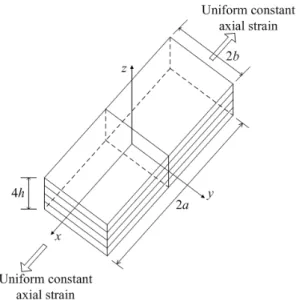
At first, free edge stress problems with a cross-ply or angle-ply lamination with four layers under uniform constant axial strain ε are considered.
Present elements capturing three-dimensional stress states are used to investigate the free edge effect. The laminated plate is shown in Fig. 2. Each of the four material layers is of equal thickness () and the laminate length and width are =80 and =8, respectively. The overall thickness is 4. The
-plane is taken to be the middle surface of the laminate with the origin of the coordinate system located at the centroid of the three-dimensional laminate. Since the geometry and loading are symmetric about the -plane, only upper half of the laminate is modeled. Thus the computational domain is defined by
≤ ≤ ; ≤ ≤ ; ≤ ≤ (15)
Also, displacement boundary conditions for the laminate are
; (16)
Location
1 2 3 4 5 6 7 8
=0 =5 1.543 1.638 1.750 1.865 1.865 1.865 2.001 2.001
= 6 1.890 1.912 1.965 1.990 2.001 2.001 2.002 2.003
=7 1.890 1.963 1.980 2.010 2.012 2.012 2.012 2.012
=8 1.890 1.963 2.012 2.012 2.013 2.013 2.013 2.013
=9 1.890 1.967 2.012 2.015 2.013 2.013 2.013 2.013
=10 1.890 1.968 2.012 2.015 2.013 2.013 2.013 2.013
Reference 1.937
<4>
2.008
<8>
2.000
<12>
2.000
<16>
2.001
<20>
2.002
<24
2.002
<24>
2.002
<24>
= =5 1.754 1.960 2.113 2.259 2.359 2.458 2.557 2.558
=6 1.800 2.008 2.114 2.271 2.344 2.449 2.550 2.559
=7 1.892 2.017 2.117 2.275 2.350 2.465 2.558 2.560
=8 1.892 2.024 2.120 2.280 2.378 2.495 2.560 2.561
=9 1.892 2.028 2.126 2.285 2.416 2.512 2.562 2.566
=10 1.892 2.030 2.128 2.286 2.426 2.586 2.563 2.569
Reference 1.462
<4>
1.790
<8>
2.017
<12>
2.180
<16>
2.307
<20>
2.411
<24
2.568
<28>
2.579
<32>
< >: The number of modeling layers
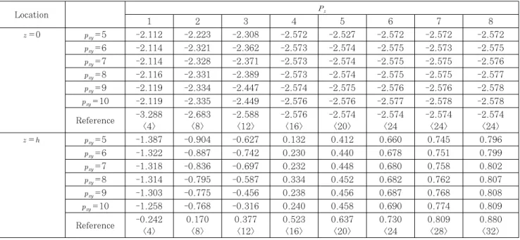
Table 1 Convergence of interlaminar normal stresses for a (0/90)s laminated plate
Location
1 2 3 4 5 6 7 8
=0 =5 -2.112 -2.223 -2.308 -2.572 -2.527 -2.572 -2.572 -2.572
=6 -2.114 -2.321 -2.362 -2.573 -2.574 -2.575 -2.573 -2.575
=7 -2.114 -2.328 -2.371 -2.573 -2.574 -2.575 -2.575 -2.576
=8 -2.116 -2.331 -2.389 -2.573 -2.574 -2.575 -2.575 -2.577
=9 -2.119 -2.334 -2.447 -2.574 -2.575 -2.576 -2.576 -2.578
=10 -2.119 -2.335 -2.449 -2.576 -2.576 -2.577 -2.578 -2.578
Reference -3.288
<4>
-2.683
<8>
-2.588
<12>
-2.576
<16>
-2.574
<20>
-2.574
<24
-2.574
<24>
-2.574
<24>
= =5 -1.387 -0.904 -0.627 0.132 0.412 0.660 0.745 0.796
=6 -1.322 -0.887 -0.742 0.230 0.440 0.678 0.751 0.799
=7 -1.318 -0.836 -0.697 0.232 0.448 0.680 0.758 0.802
=8 -1.314 -0.795 -0.587 0.334 0.452 0.682 0.762 0.807
=9 -1.303 -0.775 -0.456 0.238 0.456 0.687 0.768 0.808
=10 -1.258 -0.768 -0.316 0.240 0.458 0.690 0.774 0.809
Reference -0.242
<4>
0.170
<8>
0.377
<12>
0.523
<16>
0.637
<20>
0.730
<24
0.809
<28>
0.880
<32>
< >: The number of modeling layers
Table 2 Convergence of interlaminar normal stresses for a (90/0)s laminated plate
The 1×1 mesh composed of only one element on
-plane is considered. Due to symmetry in the layers, only two layers are required to be considered across the thickness. It means that the number of modeling layers is same with the number of physical layers of the laminate. Material properties of the layers are taken to be those of a high-modulus graphite/epoxy lamina idealized as homogeneous, orthotropic material with 137.9GPa, 14.48GPa,
5.861GPa, and ν ν ν0.21.
Convergence of the transverse normal stresses at free edge ( ) is investigated in Tables 1 and 2 for (0/90)s and (90/0)s problems, respectively. The results are compared with the values of reference (Tahani et al., 2003) which used -refinement for in-plane and out-of-plane behavior. It is seen that difference between current values with higher order shape functions and reference values with the
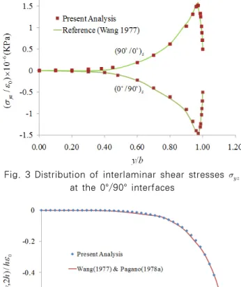
Fig. 3 Distribution of interlaminar shear stresses
at the 0°/90° interfaces
Fig. 4 Axial displacement across top surface considerable number of numerical layers is within 1%.
It is also seen that the numerical value of σ at 0°/90°
interfaces is noticeably dependent on the -refinement, not only for in-plane behavior but also for out-of-plane. Moreover, it can be stated that the transverse normal stress component grows monotonically as the order of shape functions is increased, which suggests that a stress singularity may exist at two materials interface with different fiber angles (0°/90°).
In contrast, the value of σ at the middle plane ( 0) is seen to converge to a constant value with increasing
-level. This is true because there can be no stress singularity at the interface of two layers with same fiber orientations. It is also noted that the results are practically identical for ≥6 and ≥4. In addition, both σ and σ are approximately close to zero as expected due to the symmetric nature of the cross-ply laminates.
Fig. 3 shows distribution for σ vs. at at the mid cross-section for (0°/90°)s and (90°/0°) laminates.
It is seen that the peak values of transverse shear stresses occur in the close vicinity of the free edge and then rather suddenly drop to zero at the free edge ( ). This behavior is suspected due to the presence of interfacial singularity at the free edge. Some authors (Tahani et al., 2003) argued that stress singularity may not exist at all because of nonli- nearity in the matrix material and the fact that real laminates do not exhibit distinct interfaces between layers as assumed in a macroscopic analysis. However, it is still believed by many researchers (Pipes et al., 1970; Wang et al., 1977; 1982a,b; Nguyen et al., 2006) that mathematically there is a stress singularity at the free edge at the interface of different materials.
It is to be remembered that no exact elasticity solution to the free edge problems is yet known to exist. Thus the results of present analysis are compared with the numerical solutions by Wang et al.
(1977) and excellent agreement is noted between present solutions and reference values.
Next, the prediction of free edge stresses for (45°/-45°) angle-ply laminate is considered. The finite
element mesh, boundary conditions, and material properties are identical with those of the cross-ply laminate considered last. In order to verify the present analysis for in-plane behavior, Fig. 4 shows the axial displacement distribution across the width of the top surface. Good agreement is noted between the present analysis and the references (Wang et al., 1977; Pagano, 1978).
Figs. 5 and 6 show the distribution of displacement, σ and τ along the width of the laminate at the center of the top layer. The results of present analysis and those given in the references are found to be nearly coincident for all values of . Fig. 7 shows the distribution of τ along -45°/45° interface. Contrary to the behavior noted in the case of in-plane stresses (σ and τ), absolute values of τ suddenly increase near edge of laminate, supposedly, due to free-edge effect. Moreover it is seen that the results of present
Fig. 5 Distribution of along center of top layer
Fig. 6 Distribution of along center of top layer
Fig. 7 Distribution of along -45°/45° interfaces
Fig. 8 Transverse normal stresses across the thickness (1×1 mesh)
Fig. 9 Transverse normal stresses across the thickness (2×2 mesh)
analysis for τ is closer to those of Pagano (1978) than those of Wang et al. (1977).
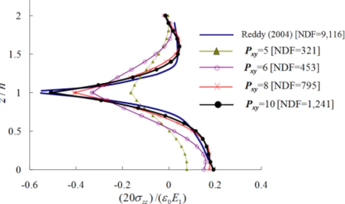
Figs. 8 and 9 show that the distributions of transverse normal stresses near the free edge (
=-0.115 and =0.998) computed by 1×1 and 2×2 mesh, respectively, and compared with the results of finite element method based on -refinement (15×5×8 mesh) (Reddy, 2004) as reference. For present
analysis, the fourth-order shape functions for out- of-plane displacement approximation were kept unchanged. It can be seen that considerable transverse normal stress develops near the interfaces with different fiber angles. It is also noticed that, in both cases, the computed results become closer to those of the reference with increasing -level. Moreover, as one will expect, the 2×2 mesh shows more rapid convergence and better qualitative agreement with the reference, while the number of degrees of freedom (NDF) used in the present model is invariably less than NDF of the reference in which conventional mesh refinement was implemented with second-order shape functions.
4.2 Laminates Undergoing Flexure
To demonstrate the effectiveness of developed finite elements for determining free-edge stresses in laminates under flexure, a simply supported (45°/-45°)s
Fig. 10 Convergence of transverse normal stresses with increase of -levels
Fig. 11 Convergence of transverse normal stresses with increase of -levels
laminated plate subjected to uniform transverse load is considered. The physical dimensions and material properties of the considered laminate are the same as in the previous axial extension example afore- mentioned if there is no specific comment. The uniform transverse load is applied to the upper surface of the laminate and acts in the negative -direction. Unlike symmetric conditions about mid- surface in the previous axial extension example, there are no planes of symmetry in this problem.
Thus the computational domain covers the entire laminate, such that
≤ ≤ ; ≤ ≤ ; ≤ ≤ (17)
The displacement boundary conditions are given by
; ;
(18)
In modeling based on -refinement, it is necessary to use highly refined mesh near free edges of interest, both in-plane and out-of-plane or thickness directions.
For modeling of present analysis, 1×1×4 mesh is considered. Thus, as in previous examples, the number of modeling layers is taken to be the same as the number of physical layers while significantly more number of discretized layers than the number of physical layers is needed in modeling based on -refinement. As discussed in the following, the results of present analysis are compared with those from reference (Reddy, 2004) using -refinement.
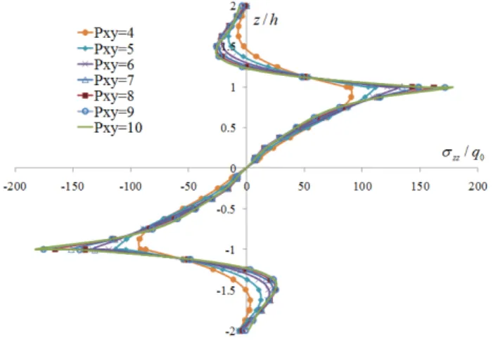
To investigate the convergence of transverse stresses, Fig. 10 shows the distribution of transverse normal stresses across the thickness at the free edge (=0, =), for increasing values of in-plane -levels () while the out-of-plane -level, , is kept unchanged at 4. In the two middle layers, both with -45° fiber angle, the responses obtained by using different are almost the same, whereas, in top and bottom layers, the nature of distribution and magnitude of transverse normal stresses across the thickness is
dependent on . It is, also, evident from the results that the transverse normal stresses in the top and bottom layers reach a converged value with increasing
, except at their interfaces with the inner layers where the values tend to increase indefinitely with
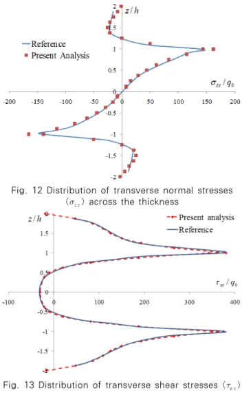
. Based on the results obtained, all stress values converged with ≥7, except at layer interfaces with different fiber angles. Fig. 11 shows distribution of transverse normal stress across the thickness with variation of -level for out-of-plane behavior (), when the -level for in-plane behavior () is kept fixed at 4. It may be noted from the results that there little difference in transverse normal stress profile when ≥4. The results in Figs. 10 and 11 are based on =8 and =4. Figs. 12 and 13 show distri- butions of transverse normal stresses and transverse
Fig. 12 Distribution of transverse normal stresses () across the thickness
Fig. 13 Distribution of transverse shear stresses ( ) across the thickness
Fig. 14 Distribution of transverse normal stresses () across the width
Fig. 15 Distribution of transverse shear stresses ( ) across the width
shear stresses across the thickness. In the two figures, the results of present analysis are compared with those of reference. It can be noted from the results that the responses by the present analysis and reference are almost same, although there is small quantitative difference in the two responses. Distribution of transverse normal stresses and transverse share stresses, at upper interfaces, across the width of the plate, for different fiber angles are shown in Figs. 14 and 15, respectively. It is seen that the results of present analysis agree well with the reference values.
It may be noted that the transverse normal stress is almost zero over the segment 0≤ 0.7, and then it rises suddenly near the free edge of the laminate.
Moreover, it can be seen that considerably high transverse shear stresses also occur over the same region, near the free edge. Thus, the results of Figs. 10 through 15
confirm the existence of singular stress field at the free edge of laminated plate under flexure.
5. Conclusions
In this study, the discrete-layer model is developed on the basis of previously -version of finite element methods for representing free-edge stresses in composite laminates. The two-dimensional-based modeling using the discrete-layer model leads to computational efficiency and acceptable accuracy. Also it makes modeling work simple considerably. On fixing mesh, the polynomial degrees of the element shape functions are increased to improve the accuracy of solution rather than the traditional approach of mesh refinement using lower- order finite elements. To predict, especially, the transverse shear stresses through the thickness of composite laminates is emphasized. It is shown that although polynomial degrees of shape functions with respect to
-plane are dominant in laminate systems, polynomial
degrees along the thickness direction have effect on accuracy of predicting interlaminar stresses. Also, it is noticed that for efficiency of analysis, different refinement levels are required with respect to
-plane and thickness. The proposed approach allows reliable investigation for existence and characteristics of free-edge stresses in composite laminates under extension and bending.
Acknowledgement
This work was supported by the Korea Research Foundation (KRF) grant funded by the Korea government (MEST)(No. 2009-0066753).
References
Ahn, J.S., Woo, K.S., Basu, P.K., Park, J.H.
(2009) Subparametric Element Based on Partial- Linear Layerwise Theory for the Analysis of Orthotropic Laminate Composites, Journal of the Computational Structural Engineering Institute of Korea, 22(2), pp.189~196..
Ahn, J.S., Basu, P.K., Woo, K.S. (2010) Analysis of Cracked Aluminum Plates with One-Sided Patch Repair Using p-Convergent Layered Model, Finite Elements in Analysis and Design, 46(5), pp.438~
448.
Babuska I., Szabo, B.A., Katz, I.N. (1981) The p-Version of the Finite Element Method, Journal of the Society for Industrial and Applied Mathematics Series B: Numerical Analysis, 18(3), pp.515~545.
Cho, M., Kim, H.S. (2000) Iterative Free-Edge Stress Analysis of Composite Laminates under Extension, Bending, Twisting and Thermal Loading, Interna- tional Journal of Solids and Structures, 37, pp.435~459.
Duster, A, Rank, E. (2001) The p-Version of the Finite Element Method Compared to an Adaptive h-Version for the Deformation Theory of Plasticity, Computer Methods in Applied Mechanics and Engineering, 190(15~17), pp.1925~1935.
Ghosh, D.K., Basu, P.K. (1998) A Parallel Progra- mming Environment for Adaptive p-Version Finite Element Analysis, Advances in Engineering Software,
29(3~6), pp.227~240.
Hong, C.H., Woo, K.S., Shin, Y.S. (1996) p-Version Finite Element Model of Stiffened Plates by Hierarchic C0-Element, Journal of the Computa- tional Structural Engineering Institute of Korea, 8(1), pp.33~45.
Hsu, P.W., Herakovich, C.T. (1977) Edge Effects in Angle-Ply Composite Laminates, Journal of Composite Materials, 11(4), pp.422~428.
Nguyen, V.T., Caron, J.F. (2006) A New Finite Element for Free Edge Effect Analysis in Laminated Composites, Computers & Structures, 84(22~23), pp.1538~1546.
Nguyen, V.T., Caron, J.F. (2009) Finite Element Analysis of Free-Edge Stresses in Composite Laminates under Mechanical and Thermal Loading, Composites Science and Technology, 69(1), pp.40
~49.
Pagano, N.J. (1974) On the Calculation of Interla- minar Normal Stress in Composite Laminate, Journal of Composite Materials, 8(1), pp.65~81.
Pagano, N.J. (1978) Stress Fields in Composite Laminates, International Journal of Solids and Structures, 14(5), pp.385~400.
Pipes, R.B., Pagano, N.J. (1970) Interlaminar Stresses in Composite Laminates under Uniform Axial Extension, Journal of Composite Materials, 4(4), pp.538~548.
Puppo, A.H., Evensen, H.A. (1970) Interlaminar Shear in Laminated Composites under Generalized Plane Stress, Journal of Composite Materials, 4(2), pp.204~220.
Ramesh, S.S., Wang, C.M., Reddy, J.N., Ang, K.K.
(2008) Computation of Stress Resultants in Plate Bending Problems Using Higher-Order Triangular Elements, Engineering Structures, 30(10), pp.2687
~2706.
Ramesh, S.S., Wang, C.M., Reddy, J.N., Ang, K.K.
(2009) A Higher-Order Plate Element for Accurate Prediction of Interlaminar Stresses in Laminated Composite Plates, Composite Structures, 91(3), pp.337~357.
Reddy, J.N. (2004) Mechanics of Laminated Composites Plates and Shells; Theory and Analysis, Second Edition, CRC Press, p.831.
Robbins Jr., D.H., Reddy, J.N. (1996) Variable Kinematic Modeling of Laminated Composite Plates,
International Journal for Numerical Methods in Engineering, 39(13), pp.2283~2317.
Rybicki, E.F. (1971) Approximate Three-Dimensional Solutions for Symmetric Laminates under Inplane Loading, Journal of Composite Materials, 5(3), pp.354~360.
Tahani, M., Nosier, A. (2003) Three-Dimensional Interlaminar Stress Analysis at Free Edges of General Cross-Ply Composite Laminates, Materials
& Design, 24(2), pp.121~130.
Wang, A.S.D., Crossman, F.W. (1977) Some New Results on Edge Effect in Symmetric Composite Laminates, Journal of Composite Materials, 11(1), pp.92~106.
Wang, S.S., Choi, I. (1982a) Boundary-Layer Effects in Composite Laminates: Part 1-Free-Edge Stress Singularities, Journal of Applied Mechanics, 49(3), pp.541~548.
Wang, S.S, Choi, I. (1982b) Boundary-layer Effects in Composite Laminates: Part 2-Free-edge Stress Solutions and Basic Characteristics, Journal of Applied Mechanics, 49(3), pp.549~560.
Woo, K.S., Basu, P.K. (1989) Analysis of Singular Cylindrical Shells by p-Version of FEM, Interna-
tional Journal of Solids and Structures, 25(2), pp.151~165.
Woo, K.S., Hong, C.H., Basu, P.K. (2003) Materially and Geometrically Nonlinear Analysis of Laminated Anisotropic Plates by p-Version of FEM, Computers
& Structures, 81(16), pp.1653~1662.
Woo, K.S., Jo, J.H., Lee, S.J. (2007) The Selective p-Distribution for Adaptive Refinement of L-Shaped Plates Subjected to Bending, Journal of the Computational Structural Engineering Institute of Korea, 20(5), pp.533~542 .
Zienkiewicz, O.C., Gago, J.P.D.S.R., Kelly, D.W.
(1983) The Hierarchical Concept in Finite Element Analysis, Computers & Structures, 16(1~4), pp.53
~65.
논문접수일 2010년 10월 25일
논문심사일
1차 2010년 11월 4일
2차 2010년 12월 6일
게재확정일 2010년 12월 7일