A Study on Accuracy Improvement of SBAS Ionospheric Correction Using Electron Density Distribution Model

1. INTRODUCTION

The users of Global Navigation Satellite System (GNSS) calculate a distance between user and GNSS satellite by using signals sent from GNSS satellites, and using the calculated distance, identify their own locations. However, since signals from GNSS satellites that arrived at user’s receivers contain many error elements such as clock error between satellite and receiver, delay, and tropospheric delay, and ionospheric delay, it is difficult to identify user’s own location accurately (Misra & Enge 2006). The largest error element among them is the ionospheric delay. The ionospheric delay can be eliminated using dual frequency but for single frequency

A Study on Accuracy Improvement of SBAS Ionospheric Correction Using Electron Density Distribution Model

Bong-Kwan Choi, Deok-Hwa Han, Dong-Uk Kim, Changdon Kee

School of Mechanical and Aerospace Engineering and the SNU-IAMD, Seoul National University, Seoul 08826, Korea

ABSTRACT

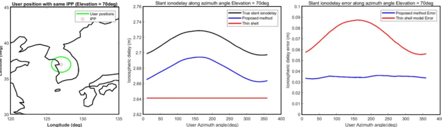
This paper proposed a method to estimate the vertical delay from the slant delay, which can improve accuracy of the ionospheric correction of SBAS. Proposed method used Chapman profile which is a model for the vertical electron density distribution of the ionosphere. In the proposed method, we assumed that parameters of Chapman profile are given and the vertical ionospheric can be modeled with linear function. We also divided ionosphere into multi-layer. For the verification, we converted slant ionospheric delays to vertical ionospheric delays by using the proposed method and generated the ionospheric correction of SBAS with vertical delays. We used International Reference Ionosphere (IRI) model for the simulation to verification. As a result, the accuracy of ionospheric correction from proposed method has been improved for 17.3% in daytime, 10.2% in evening, 2.1% in nighttime, compared with correction from thin shell model. Finally, we verified the method in the SBAS user domain, by comparing slant ionospheric delays of users. Using the proposed method, root mean square value of slant delay error decreased for 23.6% and max error value decreased for 27.2%.

Keywords: SBAS, ionospheric correction, Chapman profile, IRI, obliquity factor

users, it cannot be removed. To overcome this, a Satellite Based Augmentation System (SBAS) can be used. An SBAS provides users with ionospheric correction information, and users can calculate their location more accurately using this information.

The ionospheric correction information is generated in the master station of SBAS, at which a process that converts the slant ionospheric delay between SBAS wide area reference station and satellite, which is calculated using dual frequency, into vertical ionospheric delay is needed. Currently, SBASs employ obliquity factor of thin shell model to calculate the vertical ionospheric delay. However, a thin shell model is a method that uses only simple geometric equations without consideration of spatial changes in the ionosphere. As a result, errors exist in the vertical ionospheric delay calculated using a thin shell model from the slant ionospheric delay.

Since the ionospheric correction information in SBAS is calculated using the vertical ionospheric delay, the ionospheric correction information is inevitably inaccurate due to the aforementioned error.

To address this, the multiple shell method proposed by Received Feb 25, 2019 Revised Mar 22, 2019 Accepted May 15, 2019

†

Corresponding Author E-mail: [email protected]

Tel: +82-2-880-1912 Fax: +82-2-888-2069

Bong-Kwan Choi https://orcid.org/0000-0003-4148-2715

Deok-Hwa Han https://orcid.org/0000-0002-5549-5413

Dong-Uk Kim https://orcid.org/0000-0001-9151-4434

Changdon Kee https://orcid.org/0000-0002-8691-7068

Komjathy et al. (2002) has been employed. The method proposed by Komjathy can generate more accurate ionospheric correction information than when using a thin shell model because it can consider a vertical distribution of electron density, which a thin shell model could not do.

However, there was a drawback that the format of currently broadcast SBAS messages should be changed to apply the multiple shell method to actual SBASs (Rao 2007, Kim et al. 2015, Tao & Jan 2016). Another method was previously proposed by Hoque (Hoque & Jakowski 2013, Hoque, Jakowski & Berdermann 2014). Hoque’s method considers a vertical distribution of electron density in the ionosphere using the Chapman profile. When the vertical ionospheric delay is given through Hoque's method, GNSS users can reduce the estimated slant ionospheric delay error more efficiently than when using a thin shell model. However, since Hoque's method is a process to convert the vertical ionospheric delay into the slant ionospheric delay, it cannot be used to generate ionospheric correction information of SBAS. Thus, this study proposed a new method that can reduce estimated errors when generating ionospheric correction information of SBAS without changing the existing SBAS message structure.

2. PROPOSAL OF METHOD TO GENERATE SBAS IONOSPHERIC CORRECTION

INFORMATION

2.1 Assumptions Used in the Proposed Method

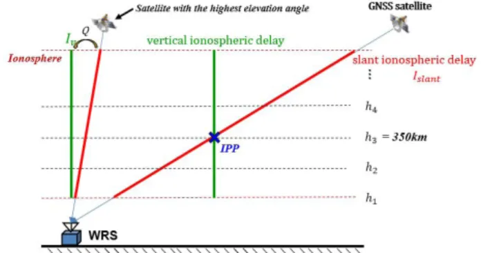
To generate ionospheric correction information in SBASs, vertical ionospheric delays at the ionospheric pierce point (IPP) are needed. To calculate the vertical ionospheric delay at the IPP, currently, SBAS uses a method that divides the slant ionospheric delay at the corresponding IPP using obliquity factor of thin shell model. However, obliquity factor of thin shell model is a function that uses only elevation without considering the spatial change in the ionosphere, thus generating estimated errors. For example, let us assume that there are line of sight (LOS) vectors that pass through the same IPP and have the same elevation. Since two vectors pass through two different paths, they have different slant ionospheric delays. However, since the elevation is the same, two vectors have the same obliquity factor, resulting in obtaining the different vertical ionospheric delays at the same IPP. When the LOS vector direction is significantly different at the nearby IPP, even if they do not pass the same IPP, there will be a significant difference in estimation of vertical ionospheric delays using the thin shell model. Since

the activities in the ionosphere environment do not change rapidly according to distance, the vertical ionospheric delay at the nearby IPP should change gradually, but it does not change gradually if the thin shell model is used. Thus, this study proposed a method to reduce the aforementioned estimated error that occurs due to the use of thin shell model when generating the ionospheric correction information in SBASs.

Hoque's study mentioned in Introduction proposed a method that calculates the slant ionospheric delay when the vertical ionospheric delay is known (Hoque & Jakowski 2013). The basic idea of the proposed method in this study was based on the algorithm proposed by Hoque. However, it is impossible to apply the algorithm proposed by Hoque simply in the opposite way to obtain the vertical ionospheric delay from the slant ionospheric delay. Thus, the algorithm proposed in this study employed the assumptions described in Table 1.

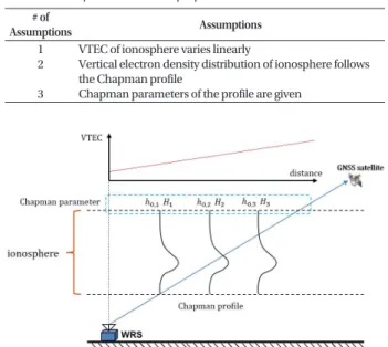
Fig. 1 is presented to help readers understand the assumptions used in the proposed method. Assumption 1 is established to supplement insufficient information to calculate the vertical ionospheric delay from the slant ionospheric delay. Through Assumption 1, a linear equation can be obtained to calculate the vertical ionospheric delay, which will be described in relation to the algorithm later.

Assumptions 2 and 3 are set to consider the change according to the horizontal difference in the ionosphere. The Chapman profile is equivalent to Eqs. (1-3) that model the vertical electron density distribution in the ionosphere (Feltens et al.

1998).

Fig. 1. Assumptions used in the proposed method.

Table 1. Assumptions used in the proposed method.

# of

Assumptions Assumptions

1 2 3

VTEC of ionosphere varies linearly

Vertical electron density distribution of ionosphere follows the Chapman profile

Chapman parameters of the profile are given

0

( , ) 1

( , , ) exp (1 exp( )) ( , ) ( )

2 2

e

N

n h z z N Chap h

eH

λ φ λ φ λ φ

π

 

=   − − −   = (1)

z h h

H

= − (2)

( ) 1 Chap h =

∫ ⁽³⁾

In Eq. (1), λ, ϕ, and h refer to the preferred longitude, latitude, and height, respectively. n

refers to the electron density at altitude h, and N

signifies the largest electron density. In Eq. (2), h

refers to the altitude where the largest electron density is located, and H refers to the atmospheric scale height. As presented in Eq. (3), a value of Chapman profile becomes 1 when integrated according to altitude.

In addition, Chapman profile can be expressed by two parameters h

and H, which are called Chapman parameters in this study. The vertical characteristics in the ionosphere can be taken into consideration by assuming the vertical electron density distribution in the ionosphere as the Chapman profile, and the horizontal characteristics in the ionosphere can also be taken into consideration by assuming that the Chapman parameters can be known.

2.2 Algorithm of the Proposed Method

The algorithm of the proposed method is described below.

Figs. 2-4 aim to help readers to understand the proposed algorithm. The equations used in the algorithm are presented in Eqs. (4-8).

( )

i v

d

I x I I

= − d + (4)

1

, ⁱ

( , , )

h

v i i h i i i

I = × I ∫

Chap h H h dh I C = ⁽⁵⁾

1

1 ,

( )

n

slant v i i

i

I

I Q f x

=

= ∑ × = ⁽⁶⁾

2

1 ( )cos(El) 1

i

RX e

i e

Q h R

h R

=

 + 

−   +  

(7)

1 1 1 2 2 2

3 3 1 1 1 2 2 2 4 4 4

(( ) ( ) )

slant v

I d d d C Q d d C Q I x dC Q d C Q d C Q d C Q

− − + − +

= + + + +



 (8)

The value to be calculated was set to x since the value that is sought by the algorithm is ultimately the vertical ionospheric delay at the IPP, and the ionosphere was divided into many layers to obtain the corresponding value. In Eq.

(4), I

refers to the vertical ionospheric delay obtained using obliquity factor of thin shell model from the slant ionospheric delay between the reference station and the satellite whose elevation is the highest among the visible satellites in the SBAS reference station. Since an error due to the thin shell model included in the vertical ionospheric delay becomes

smaller with larger elevation, the corresponding value is selected. I

refers to the vertical ionospheric delay at a place where the LOS vector between the reference station and the satellite is contacted with the i-th ionospheric layer. d refers to a distance between IPP and the reference station, and d

refers to a distance between the reference station and the i-th crossing point. The thin shell model assumes that the ionosphere is distributed at 350 km with one shell. The reason for this is because an altitude whose electron density in the ionosphere is the highest is normally near 350 km.

Thus, IPPs where the LOS vector and the thin shell model Fig. 2. Algorithm of the proposed method 1.

Fig. 3. Algorithm of the proposed method 2.

Fig. 4. Algorithm of the proposed method 3.

meet are distributed at 350 km, and the proposed method aims to calculate the vertical ionosphere delay at the IPPs as well. Thus, a distance such as d

is calculated based on 350 km. In Eq. (5), I

refers to the vertical ionosphere delay between the i-th and (i+1)-th layers, and h

refers to a distance to the i-th layer from the center of the Earth. In Eq. (6), Q

refers to the obliquity factor at the i-th layer, which can be induced using a general obliquity factor induction process as presented in Eq. (7). In Eq. (7), h

refers to a distance to the reference station from the center of the Earth, R

refers to the Earth's radius, and El refers to the elevation of the LOS vector between the reference station and the satellite. I

refers to the slant ionospheric delay between the reference station and the satellite calculated using dual frequency, which is already known. The overall procedure of the above equations expresses I

by multiplying the obliquity factor induced from the partial vertical ionosphere delay I

with regard to the i-th crossing point. Here, the change in VTEC is assumed as linear. Thus, Eq. (6) can be expressed by a linear equation about x, which is arranged to Eq. (8) to calculate the vertical ionosphere delay at the IPP.

3. VERIFICATION OF THE PROPOSED METHOD

3.1 Verification Method and Scenario

To verify the proposed method, the International Reference Ionosphere (IRI) model was used to configure the ionosphere environment. The used IRI model's dates were January 15 and October 23 of 2011, and the 20-th day of each month in 2011. There is K

Index, which is an index that influences activities in the ionosphere. The K

indexes of the 14 dates used in verification are all below three, which means all the dates had a quiet ionosphere environment. The reason why the verification was performed at such environment was because this study was basic research to improve the thin shell model and dates whose K

indexes were below three accounted for the majority at 81.6%, as shown in the investigation on K

indexes from 1932 to 2017. Fig. 5 presents the investigation results of K

index.

In addition, verification was also conducted by date in daytime (14:00), evening (18:00) and nighttime (23:00) based on Korean Standard Time (KST). The reason for this was due to the different activities in the ionosphere by time;

activities in the ionosphere were strongest at daytime when the solar activity was maximum. The reference station of the Korea Augmentation Satellite System (KASS), which was a Korean SBAS, was used to generate IPP data. Since it

was not completely constructed yet, the expected location of the reference station was employed (Authié et al. 2017).

Moreover, using broadcast ephemeris at KST 02:00, 17:00, and 22:00 on August 9, 2016 to verify the layout of various satellites, satellite orbits were generated and IPP data were obtained. Results may vary if IPP data layout differs even if one set of IRI data is used. Thus, IPP data on three dates were used for the same IRI data for verification. Accordingly, the IRI data date and the IPP data date were not matched.

The SBAS ionospheric correction information is largely divided into two steps: correction information generation step and application step of the generated correction information by SBAS users. In this study, verification for each of the two steps was conducted to verify the proposed algorithm. The results of verification at each of the steps are described below.

3.2 Verification Results of the Proposed Method at the Step Of Generating Ionospheric Correction Information

To verify the proposed method at the ionospheric correction information generation step, IRI data were used to configure an ionosphere environment. SBAS provides users with ionospheric correction information in the form of vertical ionospheric delay at the ionospheric grid point (IGP). Thus, the verification in the ionospheric correction information generation step was conducted to compare whether the vertical ionospheric delay at the IGP calculated using the proposed method had a smaller error than that using the thin shell model. For comparison, the vertical ionospheric delay calculated directly through the ionosphere environment that was configured with the IRI was set to

“true”. In addition, the slant ionospheric delay, which was

Fig. 5. Histogram of Kp index (1932.01.01 ~ 2017.12.31).

needed to calculate the vertical ionospheric delay, was also calculated using the IRI data values. Then the vertical ionospheric delay was calculated through each of the methods. The Kriging algorithm, which was employed by the

wire area augmentation system (WASS), was used to finally generate ionospheric correction information at the IGP from the vertical ionospheric delay.

Fig. 6 shows the verification result of the proposed method at the step to generate ionospheric correction information, which was executed using IRI data at 23:00 on June 20, 2011 and IPP data at 22:00 on August 9, 2016. The square in Fig.

6 indicates the pre-designated IGPs, and the color in the square signifies a level of IGP's estimated error. The red color indicates large errors whereas the blue color means smaller errors. As seen from Fig. 6, the large estimation error when using the thin shell model was alleviated by using the proposed method in this study. Tables 2-4 present the results of root-mean-square (RMS) values of the estimated errors of vertical ionospheric delay over the entire IGP shown in Fig. 6.

Since three sets of IPP data for each set of IRP data were used in the verification, three RMS values were produced. Tables 2-4 show the averaged results, in which 14 rows for each were generated because there were 14 dates for daytime, evening, Fig. 6. IGP estimation error result (IPP data: 2016.08.09 22hr (KST), IRI data: 2011.06.20 23hr (KST)) (left: thin shell model, right: the proposed method).

Table 2. Mean of RMS of vertical ionospheric delay estimation error at IGP (nighttime 23hr KST).

# of IRI data

Thin shell model (m)

Proposed method (m)

Percentage of mitigation (%) 1

2 3 4 5 6 7 8 9 10 11 12 13 14

0.41 0.64 0.92 1.14 0.57 0.68 0.53 0.73 1.68 2.06 1.63 1.19 0.40 2.02

0.39 0.60 0.87 1.12 0.47 0.45 0.40 0.68 1.67 2.15 1.72 1.28 0.38 2.10

5.6 5.6 4.9 1.3 17.5 33.4 24.1 7.4 0.7 -4.5 -5.5 -7.5 5.8 -4.1

Mean 1.04 1.02 2.1

Table 4. Mean of RMS of vertical ionospheric delay estimation error at IGP (daytime 14hr KST).

# of IRI data

Thin shell model (m)

Proposed method (m)

Percentage of mitigation (%) 1

2 3 4 5 6 7 8 9 10 11 12 13 14

2.43 3.36 3.82 4.12 4.33 3.40 3.42 3.73 4.11 4.04 3.34 2.69 2.32 4.04

1.91 2.77 3.21 3.53 3.94 3.03 2.85 3.08 3.56 3.24 2.47 1.99 1.81 3.25

21.4 17.6 16.1 14.3 8.9 10.9 16.7 17.6 13.4 19.8 26.2 26 22 19.6

Mean 3.51 2.90 17.3

Table 3. Mean of RMS of vertical ionospheric delay estimation error at IGP (evening 18hr KST).

# of IRI

data Thin shell

model (m) Proposed

method (m) Percentage of mitigation (%) 1

2 3 4 5 6 7 8 9 10 11 12 13

1.87 2.86 2.96 3.43 3.52 3.50 3.68 4.04 4.09 4.38 3.56 3.38 1.74

1.68 2.48 2.65 3.12 3.20 3.19 3.35 3.79 3.79 3.74 3.06 3.00 1.59

10.3 13.3 10.5 9.1 9.0 8.8 8.8 6.2 7.5 14.6 14.1 11.1 9.0

Mean 3.31 2.97 10.2

and nighttime. The numbers of the results were assigned according to the time order. For the evening-time result in Table 3, data on December 20, 2011, which was the last day, were omitted, thus having only 13 rows. As seen from Table 2, in terms of nighttime, estimated errors were smaller on 10

dates among the 14 dates when using the proposed method

compared to those using the thin shell model. Overall, the

error was alleviated by 2.1%, which was relatively small, and

four cases showed the results of the proposed method were

worse than that of the thin shell model. This was because

Fig. 7. Bar graph of IGP estimation error and graph of percentage of mitigation (upper: daytime, middle: evening, lower: nighttime).

the estimated error using the thin shell model was smaller in daytime than that in nighttime as a result of weaker activities in the ionosphere during nighttime. In contrast, the results of evening (Table 3) and daytime (Table 4) when the ionospheric activities were relatively strong confirmed that the estimated errors using the proposed method were smaller than those using the thin shell model, showing improvements by 10.2% and 17.3% on average, respectively. Fig. 7 shows the graph of the results presented in Tables 2-4.

3.3 Verification Results of the Proposed Method at the Step of Applying the Ionospheric Correction Information to Users

The aforementioned ionospheric correction information was applied to users and the improvements were investigated to verify the proposed method. In this verification at the user application step, a method that compared the slant ionospheric delays by changing an azimuth angle for users whose LOS vector to the satellite passed the same IPP and who had the same elevation was employed. In actual environments, it is rare for two different LOS vectors to pass the same IPP; but two different LOS vectors passing through nearby IPPs occur frequently and the occurrence frequency increases as the number of reference stations increases. As mentioned above, estimated errors occur in such environment. This study verified how many more errors could be alleviated in such environment using the proposed method than using the thin shell model. Fig. 8 shows the verification method for readers' understanding.

The slant ionospheric delay obtained directly from the ionosphere, which was configured using IRI data, was set to “true”, and the slant ionospheric delay for each method was calculated using the previously generated ionospheric correction information. Then, their differences were compared. Here, when the slant ionospheric delay was calculated using the ionospheric correction information obtained using the thin shell model, the thin shell model was employed again. However, when the slant ionospheric delay

was calculated using the ionospheric correction information obtained using the proposed method in this study, the algorithm proposed by Hoque was employed. That is, the vertical ionospheric delay at the IPP was calculated from the slant ionospheric delay (ionospheric delay between the SBAS reference station and the satellite) by employing the proposed method in this study. After this, the ionospheric correction information was generated via the Kriging method using the vertical ionospheric delay at the IPP. This process was followed by generating the slant ionospheric delay (ionospheric delay between the user and the satellite) from the vertical ionospheric delay (ionospheric correction information of SBAS), using Hoque’s method. The reason for this was because the proposed method set additional assumptions to Hoque’s method to apply the method in the opposite manner.

Table 5 presents the IPP location used in the verification, LOS vector's elevation and azimuth angle. Figs. 9 and 10 show the graphs of the slant ionospheric delays according to user's azimuth angles. The center graphs in Figs. 9 and 10 show the slant ionospheric delay results, and the blue, black, and red lines refer to the results of proposed method, true, and thin shell model, respectively. It can be seen that since the thin shell model used only obliquity factor, which was a function according to elevations, it could not follow the trend even if the azimuth angle was different for users with the same elevation. In contrast, when the proposed method and Hoque's algorithm were used, the results were found to follow the trend of true slant ionospheric delays when the LOS vector was high or low elevation. To verify whether the graph followed the trend well, RMS of the estimated error and maximum error values were numerically compared. The results are presented in Tables 6 and 7. The results in Tables 6 and 7 are depicted with graphs in Fig. 11 for readers’ visual understanding. The blue and red bars in Fig. 11 represent the results using the thin shell model and those using the proposed method in this study, respectively. As shown in Fig.

11, RMS and maximum values of the estimated errors using the thin shell model and the proposed method became larger as the elevation of the LOS vector became smaller. This was because more GPS signals passed through the ionosphere as the elevation became smaller. However, RMS and maximum values of the estimated errors for all elevations using the proposed method were smaller than those using the thin Fig. 8. Conceptual figure of the method of verification in SBAS user domain.

Table 5. Simulation configuration for verification in user domain.

Contents Value

IPP Location latitude: 37 deg longitude: 127 deg User azimuth angle

User elevation angle

0 ~ 360 deg (10 deg interval)

10 ~ 70 deg (10 deg interval)

shell model. On average, RMS and maximum values were alleviated by 23.6% and 27.2% when using the proposed method compared to when using the thin shell model. Thus, this study concluded that the results using the proposed method followed the trend of the actual slant ionospheric delay better than did those using the thin shell model.

4. CONCLUSIONS

This study was conducted to improve the accuracy when generating SBAS ionospheric correction information. To

do this, this study proposed a new method that converted slant delay to vertical delay because what could be obtained using dual frequency was the slant ionospheric delay, although the vertical ionospheric delay at the IPP was needed when generating ionospheric correction information. The proposed method employed Chapman profile and assumed that Chapman parameters were all known in order to take the spatial change in the ionosphere into consideration. The VTEC value was assumed to change linearly according to distance and the ionosphere was divided into many layers. In this manner, the vertical ionospheric delay at the IPP could be calculated by finally solving the linear equation.

Fig. 9. Slant ionospheric delay estimation result at high elevation angle (IRI data: 2011.06.20 23hr) (left: location of IPP and the user, middle: slant ionospheric delay, right: Estimation error).

Fig. 10. Slant ionodpheric delay estimation result at low elevation angle (IRI data: 2011.06.20 23hr) (left: location of IPP and the user, middle: slant ionospheric delay, right: estimation error).

Table 6. RMS of slant ionospheric delay estimation error.

Elevation

angle Thin shell

model (m) Proposed

method (m) Percentage of mitigation (%) 10

20 30 40 50 60 70

0.253 0.167 0.113 0.078 0.056 0.042 0.033

0.201 0.127 0.080 0.056 0.042 0.033 0.028

20.6 24.0 29.2 28.2 25.0 21.4 15.2

Mean 0.106 0.081 23.6

Table 7. Max error of slant ionospheric delay estimation error.

Elevation

angle Thin shell

model (m) Proposed

method (m) Percentage of mitigation (%) 10

20 30 40 50 60 70

0.416 0.265 0.175 0.121 0.089 0.066 0.049

0.311 0.193 0.121 0.084 0.063 0.048 0.038

25.2 27.2 30.9 30.6 29.2 27.3 22.4

Mean 0.169 0.123 27.2

To verify the proposed method, simulations were conducted with two steps: the first step where SBAS ionospheric correction information was generated, and the second step where the correction information was applied to users. The simulations were undertaken by configuring the ionosphere environment using IRI data. The ionospheric correction information was generated, and the results showed that the proposed method improved estimated errors by 17.3% for daytime, 10.2% for evening time, and 2.1% for nighttime. In the user application step, the proposed method followed the trend of the true slant delays better than the thin shell model did. Numerically, the proposed method improved RMS and maximum values of the estimated errors by 23.6%

and 27.2% compared to those using the thin shell model.

The method proposed in this study contributed to proposing a method that improved the thin shell model while maintaining the current SBAS message format. For future studies, the algorithm proposed in this study needs to be verified in an environment with relatively severe ionospheric activities, and the applicability of the proposed method to actual SBASs can be examined through additional verification.

ACKNOWLEDGMENTS

This research was supported by Basic Science Research Program through the National Research Foundation of Korea (NRF) funded by the Ministry of Science, ICT & Future Planning (No. NRF-2017M1A3A3A02016230), contracted through by the Institute of Advanced Aerospace Technology at Seoul National University. The Institute of Engineering Research at Seoul National University provided research facilities for this work.

AUTHOR CONTRIBUTIONS

Conceptualization, B.C., D.H. and C.K.; methodology, B.C., D.H. and C.K.; software, B.C., D.H. and D.K.; validation, B.C., D.H. and C.K.; formal analysis, B.C., D.H., D.K. and C.K.; investigation, B.C., D.H. and D.K.; resources, B.C., D.H. and D.K.; data curation, B.C., D.H. and D.K.; writing—

original draft preparation, B.C.; writing—review and editing, B.C.; visualization, B.C. and D.K.; supervision, D.H. and C.K.; project administration, B.C., D.H. and C.K.; funding acquisition, C.K.

CONFLICTS OF INTEREST

The authors declare no conflict of interest.

REFERENCES

Authié, T., Dall’Orso, M., Trilles, S., Choi, H., Kim, H., et al.

2017, Performances Monitoring and Analysis for KASS, in 2017 ION GNSS+, Portland, United States, 25-29 Sep 2017, pp.958-978. https://doi.org/10.33012/2017.15405 Feltens, J., Division, F. D., Space, E., & Centre, O. 1998,

Chapman profile approach for 3-D global TEC representation, in 1998 IGS AC Workshop, Darmstadt, Germany, 9-11 Feb 1998

Hoque, M. M. & Jakowski, N. 2013, Mitigation of ionospheric mapping function error, in 2013 ION GNSS+, Nashville, TN, 16-20 Sep 2013, pp.1848-1855

Hoque, M. M., Jakowski, N., & Berdermann, J. 2014, A new

approach for mitigating ionospheric mapping function

errors, in 2014 ION GNSS+, Tampa, Florida, 8-12 Sep

Fig. 11. Bar graph of RMS and max value of slant ionospheric estimation error and graph of mitigation percentage.

2014, pp.1183-1189

Kim, D., Han, D., Yun, H., Kee, C., Seo, S., et al. 2015, Performance Improvement of Grid Ionospheric Delay Correction Based on Multiple Constellations for Single- Frequency SBAS User, in 2015 ION Pacific PNT Meeting, Honolulu, Hawaii, 20-23 Apr 2015, pp.169-179

Komjathy, A., Wilson, B. D., Runge, T. F., Boulat, B. M., Mannucci, A. J., et al. 2002, A New Ionospheric Model for Wide Area Differential GPS: The Multiple Shell Approach, in 2002 National Technical Meeting of The Institute of Navigation, San Diego, CA, 28-30 Jan 2002, pp.460-466

Misra, B. P. & Enge, P. 2006, Global Positioning System:

Signals, Measurements and Performance, 2nd ed.

(Lincoln: Ganga-Jamuna Press)

Rao, K. N. S. 2007, GAGAN - The Indian satellite based augmentation system, Indian Journal of Radio & Space Physics, 36, 293-302

Tao, A. L. & Jan, S. S. 2016, Wide-area ionospheric delay model for GNSS users in middle- and low-magnetic- latitude regions, GPS Solutions, 20, 9-21. https://doi.

org/10.1007/s10291-014-0435-z

Bong-Kwan Choi received his B.S. and M.S.

degrees from the Department of Mechanical and Aerospace Engineering at Seoul National University in 2017 and 2019, respectively. His research interests include SBAS and ionospheric delay.

Deok-Hwa Han is a postdoctoral researcher of the GNSS Laboratory in the School of Mechanical and Aerospace Engineering at Seoul National University. He received B.S.

and Ph.D. degrees from the same university.

His recent research interests are SBAS and ionosphere modeling.

Dong-Uk Kim is a Ph.D. student in the School of Mechanical and Aerospace Engineering at Seoul National University, Republic of Korea. He received the B.S.

degree from Seoul National University in 2013. His research interests include Satellite Based Augmentation System (SBAS), network Real-Time Kinematic (RTK), and carrier-phase based algorithms for high-precision navigation system.

Changdon Kee is a Professor in the

Department of Mechanical and Aerospace

Engineering at Seoul National University

(SNU), Korea and supervises SNU GNSS Lab

(SNUGL, http://gnss.snu.ac.kr). He received

the B.S. and M.S. degrees from Seoul

National University in 1984 and 1986, and

the Ph.D. degree from Stanford University in 1994. He served

as a Technical Advisor to the Federal Aviation Administration

(FAA) on the Wide Area Augmentation System (WAAS) in

1994. His research interests include WADGPS, CDGPS,

automatic control of unmanned vehicle, and attitude

determination using GPS.