Korean Chemical Engineering Research

(1)

142 https://doi.org/10.9713/kcer.2019.57.1.142

PISSN 0304-128X, EISSN 2233-9558

Energy Stability Analysis on the Onset of Buoyancy-Driven Convection in a Horizontal Fluid Layer Subject to Evaporative Cooling

Min Chan Kim^†

Department of Chemical Engineering, Jeju National University, 102, Jejudaehak-ro, Jeju-si, Jeju-do, 63243, Korea (Received 1 September 2018; Received in revised form 14 November 2018; accepted 20 November 2018)

Abstract − The onset of buoyancy-driven convection in an initially isothermal and quiescent horizontal fluid layer was analyzed theoretically. It is well-known that at the critical Rayleigh number Ra_c= 669 convective motion sets in with a constant-heat-flux cooling through the upper boundary. Here, based on the momentary instability concept, the dimensionless critical time τm to mark the onset of convective motion for Ra > 669 was analyzed theoretically. The energy method under the momentary stability concept was used to find the critical conditions as a function of the Rayleigh number Ra and the Prandtl number Pr. The predicted critical conditions were compared with the previous theoretical and experimental results. The momentary stability criterion gives more reasonable wavenumber than the conventional energy method.

Key words: Buoyancy-driven convection, Energy stability, Relative energy, Momentary stability

1. Introduction

Buoyancy-driven convection plays an important role in many engineering problems, such as chemical vapor deposition, solidification, electroplating, and also conventional heat and mass transfer systems. Most of these processes involve nonlinear developing temperature profile, so it becomes important to predict when the buoyancy-driven convection sets in. But a general approach to predict the critical conditions to mark the onset of buoyancy-driven convection under these circumstances is still under controversy.

When an initially quiescent, horizontal fluid layer is cooled from above or heated rapidly from below, the basic temperature profile of heat conduction develops with time and buoyancy-driven convection setting in at a critical time. In this transient system, the critical time tc to mark the onset of convective motion becomes an important question, which may be called an extension of classical Rayleigh- Bénard problems. The related instability analyses have been conducted under linear stability theory and nonlinear energy method. Based on the linear stability theory, the frozen-time model [1], amplification theory [2] and propagation theory [3] have been derived and applied to the various systems. Homsy [4], Gummerman and Homsy [5], and Wankat and Homsy [6] applied the nonlinear energy method to ana- lyze this kind of problem. Straughan [7] summarized the theoretical aspects of the energy method for the various systems. Also, Harfash and Straughan [8] used the energy method to study the magnetic

field effect on the convective instability.

Based on the relative stability concept, Kim and colleagues [9-14]

analyzed the energy stability of the various systems. Their relaxed energy method gives the critical time tc for the whole range of Pr and Pa, but the conventional energy method yields the stability criteria independently of Pr. Here we concentrated on the instability problem in an initially isothermal, quiescent fluid layer. Starting from time t = 0, the upper free boundary is cooled uniformly by evaporation. For this specific system, the stability criteria were obtained based on the original energy method and its modification, and they were compared with available experimental and theoretical results.

2. Theoretical analysis 2-1. Governing equations and base system

The system considered here is a Newtonian fluid layer with an initial temperature. For time t ≥ 0, the horizontal layer of fluid depth, d, experiences evaporative cooling with heat flux, q, through the upper free boundary, and its lower boundary is kept at the initial temperature, Ti. A schematic diagram of the basic system of pure conduction is shown in Fig. 1. For a high q, buoyancy-driven convection will set in at a certain time, and the governing equations of flow and temperature fields are expressed by employing the Boussinesq approxi- mation as

, (1) , (2)

, (3) where is the velocity vector, ρ the density, P the

0

=

⋅

∇ U

( )

{ }

1 P 2 1 T Ti

t

⎧∂+ ⋅∇⎫ = − ∇ + ν∇ + −β −

⎨∂ ⎬ ρ

⎩ U ⎭U U g

T t T

∇2

α

⎭ =

⎬⎫

⎩⎨

⎧ + ⋅∇

∂∂ U

( )

(

⁼ ^{U ,}^,^V^W

)

U

†To whom correspondence should be addressed.

E-mail: [email protected]

‡This article is dedicated to Prof. Lae Hyun Kim on the occasion of his retire- ment from Seoul National University of Science & Technology.

This is an Open-Access article distributed under the terms of the Creative Com- mons Attribution Non-Commercial License (http://creativecommons.org/licenses/by- nc/3.0) which permits unrestricted non-commercial use, distribution, and reproduc- tion in any medium, provided the original work is properly cited.

(2)

dynamic pressure, ν the kinematic viscosity, T the temperature, g the gravitational acceleration, β the thermal expansion coefficient, and α the thermal diffusivity.

Let’s assume the evaporation rate and corresponding heat flux q are constant. The validity of this assumption will be discussed later.

Then, the basic state of heat conduction the dimensionless temperature profile is represented by [15].

, (4)

with the following initial and boundary conditions,

θ₀= 0 at τ = 0 and z = 1, (5a)

at z = 0, (5b) where τ = αt/d², z = Z/d and θ0= k(T-Ti)/(qd). Here, k is the thermal conductivity of the fluid. The subscript ‘0’ denotes the basic state. The exact solution of Eqs. (4) and (5) is well-known:

, (6a)

, (6b)

where , , and . Equa-

tion (6b) is obtained in terms of the integral of complementary error functions by using the Laplace transform.

2-2. Stability equations

Consider the following velocity, pressure and temperature perturbations: U₁= U−U0, P₁= P−P0 and T1= T−T0, and let’s intro- duce these perturbations into Eqs. (1)-(3). Then, using α/d, ρα²/d², and qd/k as the scaling factors of velocity, pressure and temperature, respectively, we can obtain the following dimensionless equations:

, (7) , (8)

, (9)

under the following boundary conditions:

at z = 0, (10a) at z = 1, (10b)

where k is the unit vector of the positive z-direction, and subscripts 0 and 1 represent the base and perturbation quantities, respectively.

Here, and are the Prandtl num-

ber and the Rayleigh number, respectively.

Now, multiply Eq. (8) by u₁ and Eq. (9) by θ1 and integrate over the system volume Ω, then Eqs. (8) and (9) become,

, (11) . (12) Using the divergence theorem, the following relations can be obtained:

, (13)

, (14)

where , and . In above der-

ivation, the boundary condition of Eq. (10) and the periodicity in x- and y-direction are used.

In the present system the dimensionless natural energy can be defined as a linear combination of Eqs. (13) and (14) with the cou- pling constant γ > 0:

(15)

and the following energy identity can be derived

(16)

where w1 is the vertical component of the velocity perturbation vector and the primes are dropped for the sake of simplicity. By setting , the above energy identity can be expressed as

(17)

where . After dropping the hats, the above relation can be represented as

(18)

20 0 2

∂z θ

=∂

∂τ

∂θ

0 =−1

∂

∂θ z

(

⁻^μ ^τ

)

μ μ

−

=

θ⁰ ¹ ²

∑

_n^∞₌₁ ¹ ^cos⁽ ⁿ ⁾^exp ⁿ²

n

z z

∑

^∞

= ⎭⎬⎫

⎩⎨

⎧ ⎟⎟⎠⎞

⎜⎜⎝⎛ −ζ τ

− +

⎟⎟⎠⎞

⎜⎜⎝⎛ +ζ

− τ τ

= θ

0

*0 2

ierfc 1 ierfc 2

) 1 ( 4

n

n n n

( )

^τ ⁼^θ

( )

^τ^ζ

θ₀ ,z ^*₀ , ^μn⁼

(

ⁿ⁻¹²

)

^π ζ z= τ

1=0

⋅

∇ u

1 1 2 1 1

1 1 =−∇ +∇ + θ

⎭⎬

⎫

⎩⎨

⎧ + ⋅∇

τ

∂

∂ p Ra

Pr u u u k

1 0 1

1 2 1

1 − ⋅∇θ

∂ θ

− ∂ θ

∇ τ =

∂ θ

∂ u

w z

0

1 1 =

∂ θ

=∂ u z

1 0

1=θ = u

( )

Pr = ν α ^Ra

{

^{= β}^{g qd}⁴

(

^k^αν

) }

Ω θ + Ω

∇

⋅ +

⎟ Ω

⎠

⎜ ⎞

⎝⎛ +

∇

⋅

−

= τ Ω

∂

∫ ∫ ∫

∫

_Ω _Ω _Ω

Ω

d w Ra d d

p

Pr d ¹ ¹ ¹

1 2 12

1 1 12

2 1 2

1 u u u u u

∫

_Ω _Ω _Ω

Ω

∂ Ω θ θ ∂

− Ω θ

∇ θ + Ω θ

∇

−

= τ Ω

∂ θ

∂ d

w z d d

d 2 1 1 1 ⁰

1 1

1 12

2

1 u

1 1 2 1 2

1 1

2

1 =− ∇ + θ′

τ

∂

∂ Rw

Pr u u

w z

R ∂

θ θ′∂

− θ′

∇

− τ =

∂ θ′

∂ 0

1 1 2

1 2

1

2 1

R= Ra θ1′= Raθ1 〈 〉( ). ( ) Ω. d

Ω

∫

=

( )

1 ²

2

1 2

1 Pr

2

1 + γθ′

=

τ u

E

2 1 1 1 0 1

1 2

1 θ + θ − ∇u

∂ θ γ ∂

− θ

∇ γ

− τ =

∂

∂ R w

w z E R

1

ˆ1= γθ θ

0 1 1 1

1 2 1 2

1 ˆ ˆ

ˆ ˆ

θ

∂ γ θ

− ∂ γ + θ

∇ + θ

∇

− τ =

∂

w z w

E u R

2 1 2

1 ˆ

2 1 2

ˆ= 1 u + θ

E Pr

1 dE RI D d

D I R

D

= − τ

⎛ ⎞

= − ⎜⎝ − ⎟⎠ Fig. 1. Sketch of the basic conduction state considered here.

(3)

where

(19)

. (20) Even though we can describe the temporal evolution of the perturbation energy through Eq. (18), care must be taken in defining the stability criterion for the system having time-dependent base states.

Shen [16] first observed, in a study of time dependent parallel shear flow, if the kinetic energy of a perturbation decreases in time but that of the base state decreases at a faster rate, then the kinetic energy of perturbation will appear amplified in time. Conversely, if the kinetic energy of the perturbation increases in time but that of the base state increases faster still, then the kinetic energy of the perturbation will appear to decay in time. To determine the stability characteristics of perturbations of time variant base states, Shen [16] introduced the concept of “momentary stability” where the stability of the system is guaranteed if

, (21)

where

(22)

is called the relative energy [17] and the momentary stability has been known as relative stability [18]. Here E and E0 are the energy of the disturbance and that of base state, respectively. For the present system, E0 is defined as

. (23)

With these definitions, the criterion for momentary stability of unsteady base state is given by

. (24)

Here σ and σ0 are the growth rate of the disturbance and that of base energy defined as

and . (25)

For the present system, based on Eq. (6a) the growth rate of base energy is

. (26)

For the limiting case of τ→∞, σ0→0 is obtained.

It is well-known that the present system with Ra > 669 is asymp- totically unstable [19]. Therefore, our primary concern is the instan-

taneous instability, which is defined as

, (27)

under the momentary instability concept [16]. The neutral stability condition under the momentary instability can be determined from

. (28) And, therefore the momentary stability limit can be obtained as

. (29)

under the condition of

= 1. (30)

This maximum problem can be solved by the variational tech- nique. And, under the normal mode analysis, the following Euler- Lagrange equations can be obtained:

, (31) (32)

under the following boundary conditions:

at z = 0, (33a)

at z = 1, (33b)

The momentary stability limit Ra is given by

(34)

Since σ0→0 as τ→∞, for the limiting case of large τ, the above stability equations degenerate into the conventional strong stability equations.

3. Solution Method

The stability equations (31)-(33) were solved by employing the outward shooting scheme [20]. To integrate them, trial values of the eigenvalue R and the boundary conditions d³w1/dz³ and θ1 at z = 0 are assumed properly for a given a and γ. Since the boundary condition, Eq. (33) are all homogeneous, the value of dw1/dz at z = 0 can be assigned arbitrarily. This procedure is based on the outward shooting method in which the boundary value problem is transformed into the initial value problem. The trial values, together with the three known conditions at the lower boundary, give all the information to make numerical integration smooth.

The integration based on the 4th-order Runge-Kutta method is

0 1 1 1

1 λθ

∂ θ

− ∂ λ

= θ

w z w I

2 1 2

1 +∇u

θ

∇

= D

0 τ <

d dER

E0

ER= E

⎭⎬

⎫

⎩⎨

⎧ θ

=

∫

¹

0 20

0 2

1 dz E

0

1 =σ−σ dτ

dE E

R R

= τ

σ d

dE E 1

= τ

σ d

dE E

0 0

0 1

( ) ( ) { ( ) }

∑

∞

=

∞

=

τ μ

−

− τ μ

− μ

−

τ μ

−

− τ μ

− μ

= σ

1

2 2

4 1

2 2

4

0

exp 2 exp 16 24 1

exp 1 exp 8

n n n n

σ0

>

σ

σ0E=RI D–

⎥⎦

⎢ ⎤

⎣

⎡ σ

= +

E D

I

R 0

1 max

2 1 2

1 +∇u

θ

∇

= D

2 1 2 0 2 2 1 1 0

2 2 2 2

2 1

2

1 a w

dz d a Pr

R z w dz a

d ⎟⎟⎠⎞

⎜⎜⎝⎛ − + σ

⎟ θ

⎟

⎠

⎞

⎜⎜

⎝

⎛

∂ θ γ∂ γ−

−

⎟⎟⎠ =

⎜⎜⎝ ⎞

⎛ −

0 1 0 1 2 1

2 2

2 1

2

1 ⎟⎟ +σ θ

⎠

⎞

⎜⎜

⎝

⎛

∂ θ γ∂ γ−

=

⎟⎟⎠θ

⎜⎜⎝ ⎞

⎛ − w

R z dz a

d

1 0

2 2 1

1= = θ =

dz d dz

w w d

1 0

1= 1 =θ =

dz w dw

R Ra maxmin_a

= γ

(4)

performed from z = 0 to z = 1. By using the Newton-Raphson itera- tion the trial values of R, d³w1/dz³, and θ₁ are corrected until the stability equations satisfy the upper boundary conditions within the relative tolerance of 10^-10. For the strong stability limits, the solution procedure is almost the same as above.

4. Results and Discussion

Since, for large τ, the base temperature field becomes linear and therefore σ₀→0, the present momentary stability degenerates to the conventional energy method. For this case, the critical condition is Ra = 669 [19]. The present stability limits given in Fig. 2 reconstruct this condition. By employing the momentary stability concept, we tried to relax the conventional energy method and to reanalyze the well-known transient Rayleigh-Bénard problem. The present relaxation can show the Prandtl number effect on the stability conditions, which has been ignored in the original energy method based on the strong stability criterion. The present relaxation shows that the critical time τm based on the momentary stability concept decreases with an increase in Ra and also Pr. The Pr-effect becomes pronounced for Pr < 1, which means the inertia term in Eq. (31) makes the system more stable.

For the isothermally heated system, Neitzel [21] reported the global stability limits under the conventional energy stability method. The global limits are Ra = 1699 (at ) and 1013 (at ) for the rigid-rigid boundaries system and free-rigid boundaries one, respectively. This global stability limits are lower than the asymp- totic stability limits, which are 1708 and 1101, respectively. However, this global minimum cannot be shown in the rigid-free boundaries system. The free-rigid boundaries system corresponds to rigid-free boundaries system cooled from free, upper boundary, which is similar situation to the present system. Kim et al. [13] reconsidered this problem using the relative stability criterion. According to their results, the global minimum was not observed for the various boundary situations. And, as shown in Fig. 2, the present system does not

show the global minimum. Therefore, the global minimum phenom- ena seem to be dependent on the boundary conditions, heating or cooling history and stability criteria.

Wankat and Homsy [6] analyzed the stability condition and sug- gested the minimum bound of stability of the system similar to the present one. However, they simulated the evaporative cooling as the ramp cooling rather than the present constant flux cooling and used free-free boundary conditions for the upper and lower boundaries.

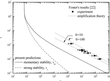
Furthermore, they employed the strong instability criterion σ > 0 rather than present momentary instability σ > σ₀ as an instability criterion. They compared their results with Foster’s [22] experiments for water layer, where the top boundary was cooled by evaporation.

Manifest convection was detected first at t = to by visual observation of the motion of a thin layer of ink near the bottom layer. The typical surface temperature record, Figure 2 of Foster’s, might be represented well by the constant flux cooling model, , rather than the ramp cooling one, . In the present study the experimental data are converted,

, (35)

where is the Rayleigh number defined by Foster based on the cooling rate φ. Due to the differences described above, direct comparison with Wankat and Homsy’s [6] work is not possible.

Foster [22] analyzed the stability limits using the amplification theory based on the ramp cooling model. In comparing his predic- tion with his experimental data, he argued that the amplification of the initial disturbances of somewhere between 10 and 100 is neces- sary for the detection of manifest convection, as shown in Fig. 3. He defined the amplification factor as the ratio of the root-mean- square quantity of velocity disturbances at t = to to that of the assumed white-noise ones at t = 0. But we do not know what initial conditions exist in nature. In Fig. 3, the present predictions are compared with Foster’s theoretical and experimental work. The present predictions

1 2 2 0 2

2 a w

dz d

Pr ⎟⎟⎠⎞

⎜⎜⎝⎛ − σ

τ 0.14≈ τ 0.08≈

(

^Ts−^Ti

)

~ ^t

(

^Ts−^Ti

)

~^t

( )

⁰

ierfc 4τ

=

φτ Ra

Ra

( )

^α ^ν

βφ

φ =g d5 2

Ra

w

Fig. 2. Effect of Pr on the stability condition. Fig. 3. Comparison of critical Rayleigh numbers with previous results.

(5)

are quite different from the experimental data. However, the present momentary stability criterion is much closer to the experimental data than the conventional strong stability criterion. The quantitative dis- crepancy between the experimental data and the predictions based on the energy method is of foreknowledge, since the energy methods need not satisfy the dynamical equations which describe the actual experimental process. Therefore, the energy methods have been employed as lower bounds of stability. Since no experimental data lie to the left of the energy stability limits, the present predictions do not commit the theoretical base point. It is well-known that the energy method cannot give the information on the crtical wave number. However, the present modification gives a reasonable wavenumber at the onset of convection. As shown in Fig. 4, the present momentary stability criterion gives a more reasonable wavenumber than the original energy method, where the critical wavenumer is ac= 2.08 for the whole range of Ra.

5. Conclusions

The critical condition to mark the onset of convective motion driven by buoyancy forces in an initially quiescent, horizontal layer cooled from above was analyzed based on the energy method. By considering the growth rate of the relative energy, we modified the conventional energy method. Based on the present modification, we defined the momentary stability time τm from which the growth rate of the perturbation energy exceeds that of the base energy. The present modification predicts experimental trends which cannot be explained by the original energy method.

Since the energy methods need not satisfy the dynamical equations such as Navier-Stokes equation and the heat transport equation, the growth of disturbance should be studied by solving dynamical governing equations fully.

Acknowledgments

This research was supported by the 2018 scientific promotion pro- gram funded by Jeju National University.

References

1. Morton, B. R., “On the Equilibrium of a Stratified Layer of Fluid,” J. Mech. Appl. Math., 10, 433(1957).

2. Foster, T. D., “Stability of Homogeneous Fluid Cooled Uni- formly From Above,” Phys. Fluids, 8, 1249(1965).

3. Ryoo, W. S. and Kim, M. C., “Effect of Vertically Varying Per- meability on the Onset of Convection in a Porous Medium,”

Korean J. Chem. Eng., 35, 1247(2018).

4. Homsy, G. M., “Global Stability of Time-Dependent Flows:

Impulsively Heated or Cooled Fluid Layers,” J. Fluid Mech., 60, 129(1973).

5. Gumerman, R. J. and Homsy, G. M., “The Stability of Uniformly Accelerated Flows with Application to Convection Driven by Surface Tension,” J. Fluid Mech., 68, 191(1975).

6. Wankat, P. C. and Homsy, G. M., “Lower Bounds for the Onset Time of Instability in Heated Layers,” Phys. Fluids, 20, 1200 (1977).

7. Straughan, B., The Energy Method, Stability, and Nonlinear Convection, 2^nd ed. Applied Mathematical Sciences, vol. 91. New York, NY: Springer (2004).

8. Harfash, A. J. and Straughan, B., “Magnetic Effect on Instabil- ity and Nonlinear Stability in a Reacting Fluid,” Meccanica, 47, 1849(2012).

9. Kim, M. C. and Choi, C. K., “Energy Stability Analyses on the Onset of Convection Driven by Soret-Effect in Nanoparticles Suspension Heated from Above,” Phys. Rev. E., 76, 036302(2007).

10. Kim, M. C. and Choi, C. K., “Relaxed Energy Stability Analysis on the Onset of Buoyancy-Driven Instability in the Horizontal Porous Layer,” Phys. Fluids, 19, 088103(2007).

11. Kim, M. C., Choi, C. K., Yoon, D. Y. and Chung, T. J., “Onset of Marangoni Convection in a Horizontal Fluid Layer Experi- encing Evaporative Cooling,” Ind. Eng. Chem. Res., 46, 5775(2007).

12. Kim, M. C., Song, K. H. and Choi, C. K., “Energy Stability Analysis for Impulsively Decelerating Swirl Flows,” Phys. Fluids, 20, 064101(2008).

13. Kim, M. C., Choi, C. K. and Yoon, D.-Y., “Relaxation on the Energy Method for the Transient Rayleigh-Bénard Convection,” Phys.

Lett. A, 372, 4709(2008).

14. Kim, M. C., “Onset of Buoyancy-Driven Convection in Isotro- pic Porous Media Heated from Below,” Korean J. Chem. Eng., 27, 741(2010).

15. Vidal A. and Acrivos A., “Effect of Nonlinear Temperature Pro- files on Onset of Convection Driven by Surface Tension Gradi- ents,” Ind. Eng. Chem. Fundamen., 7, 53(1968).

16. Shen, S. F., “Some Considerations on the Laminar Stability of Time-Dependent Basic Flows,” J. Aero. Sci., 28, 397(1961).

17. Matar, O. K. and Trojan, S. M., “The Development of Transient Fingering Patterns During the Spreading,” Phys. Fluids, 11, 3232 (1999).

18. Chen, J.-C., Neitzel, G. P. and Jankowski, D. F., “The Influence Fig. 4. Comparison of the critical waver number with the experi-

mental results.

(6)

of Initial Condition on the Linear Stability of Time-Dependent Circular Couette Flow,” Phys. Fluids, 28, 749(1985).

19. Davis, S. H., “Buoyancy-Surface Tension Instability by the Method of Energy,” J. Fluid Mech., 39, 347(1969).

20. Hwang, I. G., “On Compositional Convection in Near-Eutectic Solidification System Cooled from a Bottom Boundary,” Korean

Chem. Eng. Res., 55, 868(2017).

21. Neitzel, G. P., “Onset of Convection in Impulsively Heated or Cooled Fluid Layers,” Phys. Fluids, 25, 210(1982).

22. Foster, T. D., “Onset of Convection in a Layer of Fluid Cooled from Above,” Phys. Fluids, 8, 1770(1965).