2006, Vol. 17, No. 4, pp. 1343 1348 2006, Vol. 17, No. 4, pp. 1343 1348 2006, Vol. 17, No. 4, pp. 1343 1348 2006, Vol. 17, No. 4, pp. 1343 1348~~~~
Truncated Point and Reliability Truncated Point and ReliabilityTruncated Point and Reliability Truncated Point and Reliability
in a Right Truncated Rayleigh Distribution in a Right Truncated Rayleigh Distribution in a Right Truncated Rayleigh Distribution in a Right Truncated Rayleigh Distribution
Joongdae Kim Joongdae Kim Joongdae Kim Joongdae Kim1)1)1)1)
Abstract Abstract Abstract Abstract
Parametric estimation of a truncated point in a right truncated Rayleigh distribution will be considered. The MLE, a bias reduced estimator and the ordinary jackknife estimator of the truncated point in the right truncated Rayleigh distribution will be compared by mean square errors.
And proposed estimators of the reliability in the right truncated Rayleigh distribution will be compared by their mean squared errors.
Keywords Keywords Keywords
Keywords : Jackknife, Reliability, Right truncated Rayleigh distribution
1. Introduction 1. Introduction 1. Introduction 1. Introduction
Here we shall consider a right truncated Rayleigh distribution with the following pdf:
, where >0. (1.1)
The right truncated Rayleigh distribution has an increasing failure rate, ideally suited for use as a survival distribution for biological and industrial data.
For values of a truncated point η that are corresponding to small amounts of truncation, the hazard rate function increases very slowly up to a certain time and then asymptotically climbs to infinity at the truncated point η.
Hannon & Dahiya(1999) examined the general and asymptotic properties of all estimators in a right truncated exponential distribution . Kim(2006), Lee(2006), and
1) Associated Professor, Department of Computer Information, Andong Sciences College Andong, 760-300, Korea
E-mai : [email protected]
Lee & Won(2006) studied inferences on reliability in an exponentiated uniform distribution and an exponential distribution.
Here the MLE, a bias reduced estimator and the ordinary jackknife estimator of the truncated point η in the right truncated Rayleigh distribution will be considered, and we shall compare three estimators of η in a sense of MSE.
And proposed estimators of reliability in the right truncated Rayleigh distribution will be compared each other in a sense of MSE
2. Truncated Point Estimation 2. Truncated Point Estimation2. Truncated Point Estimation 2. Truncated Point Estimation
From the pdf (1.1) of the right truncated Rayleigh distribution and formula 8.250(1) in Gradsheyn & Ryzhik(1965), its k-th moment can be obtained:
′ ≡
′ , k=1,2,... (2.1)
where , ′ and ′ ≡ .
Let be a simple random sample from the right truncated Rayleigh distribution with the pdf (1.1). Then, from the Factorization Theorem in Rohatgi(1976), the largest order statistics is a sufficient statistic, its pdf is given by:
⋅ ⋅ ⋅ , 0<x< (2.2) where .
From the formulas 3.381(1), 8.356(1), 8.359(4) & 0.155(3) in Gradsheyn &
Ryzhik(1965) and the pdf (2.2) of , we can obtain Ist and second moments of the largest order statistics :
⋅
⋅ ⋅ , and
(2.3)
where and
.
The (n-1)th order statistics has the following pdf:
, 0<x< (2.4)
where .
From the formulas 8.381(1), 8.359(4), 3.38191) and 0.155(3) in Gradsheyn &
Ryzhik(1965) and the pdf (2.4) of , we can obtain Ist and second moments of the (n-1)th order statistics :
, and
+ . (2.5)
where and
.
The joint pdf of the two order statistics and is given by:
, 0<x<y< (2.6)
where .
Let ≡ be defined, where k is non-negative integer Then, by the formula 6.287(1) in Gradsheyn & Ryzhik(1965), the integral I(k) converges.
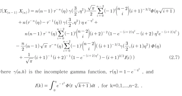
From the joint pdf (2.6) and the formulas 3.381(1), 8.356(1) and 8.350(4) in Gradsheyn & Ryzhik(1965), we can obtain the following expectation
(2.7)
where is the incomplete gamma function, , and
≡ , for k=0,1,...,n-2, .
The following estimators of the truncated point η of the pdf(1.1) in the right truncated Rayleigh distribution are given as the followings:
, the MLE of η,
, a bias reduced estimator of (Hannon &
Dahiya(1999)), and
, the ordinary jackknife estimator of (Gray & Schucany(1972)).
From the expectations (2.3), (2.5) and (2.7), we can obtain the expectations and variances of estimators MLE , a bias reduced estimator , and the ordinary jackknife estimator .
Table 1 shows numerical MSE of three estimators of a truncated point in the right truncated Rayleigh distribution when n=10(10)50 and =1.
<Table 1> MSE of MLE, a bias reduced estimator and the ordinary jackknife estimator when =1.(units are )
sample size
10 9.5151 9.7467 8.8562
20 3.3120 3.0695 2.9580
30 1.3385 1.5411 1.4821
40 0.7983 0.8131 0.7928
50 0.5323 0.5493 0.4994
Through Table 1, we can obtain the following estimation for the truncated point.
Fact 1. When n=10(10)50 and =1,
(a) The ordinary jackknife estimator is more efficient than other two estimators.
(b) The bias reduced estimator is more efficient than the MLE .
3. Reliability Estimation 3. Reliability Estimation3. Reliability Estimation 3. Reliability Estimation
Based on the pdf (1.1) of the right truncated Rayleigh distribution, its right tail probability(or reliability) in the right truncated Rayleigh distribution is
⋅ , where ≡ . Since
⋅ ⋅ is positive for >0 , is a monotone increasing function of .
Therefore, inference on η is equivalence to inference on (see McCool(1991)), and so it's sufficient for us to estimate η instead of estimating
(see McCool(1991)).
Here we could recommend the ordinary jackknife estimator of to estimate
by the results in Section 2.
Next we shall consider estimation of
instead of estimating
=1- .
From the MLE of η, the MLE of F(t) is given by:
⋅ , 0<t< η, where .
From the pdf (2.2) of , we can obtain the expectation and variance of
:
and
. (3.1)
From the expectation in the result (3.1),
≡
⋅ , 0<t< η, where
is an unbiased estimator of F(t), and its variance is
. (3.2)
From the results (3.1) and (3.2), is less than . we can obtain the following:
Fact 2. An unbiased estimator is more efficient then the MLE in a sense of MSE.
While, for non-parametric estimation F(t), we have well known the followings in Rohatgi(1976)
#{≤ , for i=1,2,...,n } /n
and =F(t)(1-F(t))/n. (3.3) From the results (3.2) and (3.3), we can obtain :
Fact 3. An unbiased estimator is more efficient than the non-parametric estimator in a sense of MSE for all t satisfying F(t)<
, vice versa for else t.
References References References References
1. Gradsheyn, I. S. & Ryzhik, I. M.(1965), Tables of Integral, Series, and Products, Academic Press, New York.
2. Gray, H. L. & Schucany, W. R. (1972), The Generalized Jackknife Statistic, Markel Decker, Inc., New York.
3. Hannon, P. M. & Dahiya, R. C.(1999), Estimation of Parameters for the truncated Exponential Distribution, Commun. Statist.-Theory Meth., 28(11), 2591-2612.
4. Kim, J.(2006), The UMVUE of [P(Y>X)]k in a Two Parameter Exponential Distribution, J. of the Korean Data & Information Science Society 17-2, 493-498.
5. McCool, J. I.(1991), Inference on P(X<Y) in the Weibull Case, Commun.
Statist.,-Simula., 20(1), 129-148.
6. Lee. J. (2006), Reliability and Ratio of two Independent Exponential Distribution, J. of the Korean Data & Information Science Society 17-2, 515-520.
7. Lee, C. & Won, H.(2006), Inference on Reliability in an Exponentiated Uniform Distribution, J. of the Korean Data & Information Science Society 17-2, 507-514.
8. Rohatgi, V. K.(1976), An Introduction to Probability Theory and Mathematical Statistics, John Wiley & Sons, New York.
[ received date : Sep. 2006, accepted date : Nov. 2006 ]