Bayesian Estimation Using Noninformative Priors in Hierarchical Model

(1)

2004, Vol. 15, No. 4, pp. 1033∼1043

Dal Ho Kim¹⁾․Jin Kap Choi²⁾․Hee Jo Choi³⁾

Abstract

We consider the simultaneous Bayesian estimation for the normal means based on different noninformative type hyperpriors in hierarchical model.

We provide numerical example using the famous baseball data in Efron and Morris (1975) for illustration.

Keywords : Bayesian estimation, hierarchical model, matching priors, normal means

1. Introduction

Bayesian methods have become increasingly popular in the theory and practice of statistics. This is partly due to the fact that even with little or no prior information, one can often employ noninformative priors to draw reliable inference.

In practice, empirical and hierarchical Bayes methods are useful, especially in the context of simultaneous estimation of several parameters.

For example, agencies of the federal government have been involved in obtaining estimates of per capita income, unemployment rates, crop yields and so forth simultaneously for several state and local government areas. In such situations, quite often estimates of certain area means, or simultaneous estimates of several area means can be improved by incorporating information from similar neighboring areas. Examples of this type are especially suitable for empirical Bayes (EB) and hierarchical Bayes (HB) analyses.

EB and HB methods are being routinely used whenever there is a need to 1) First Author : Associate Professor, Department of Statistics, Kyungpook National

University, Taegu, 702-701, Korea E-Mail : [email protected]

2) Professor, Department of Statistics, Kyungpook National University, Taegu, 702-701, Korea

3) M.S., Department of Statistics, Kyungpook National University, Taegu, 702-701, Korea

(2)

"borrow strength" either for inference related to a particular parameter of interest, or simultaneous inference for several parameters. In particular HB methods are gaining increasing popularity in recent years partly due to overcoming the difficulty in calculation even if we use vague or noninformative priors. Thus, not surprisingly, over the years, a wide range of noninformative priors has been proposed and studied. One popular criterion for the development of such priors is to match asymptotically the posterior coverage probability of a Bayesian credible set with the corresponding frequentist coverage probability.

The outline of this paper is as follows. In Section 2, we introduce a matching prior for the hyperparameter in the normal HB model following Datta, Ghosh and Mukerjee (2000). This prior turns out to be different from the one proposed by Morris(1983). In Section 3, we derive expressions for the posterior means and variances with different hyperpriors in the normal HB setup. And in Section 4, we provide numerical example using the famous data of Efron and Morris(1975) for illustration.

2. Matching Priors in Hierarchical Model

We consider the following normal HB model

Ⅰ. Y_i| θ_i, μ, τ² ∼ ind N( θ_i, σ²), i = 1,..., n ;

Ⅱ. θ_i| μ, τ² ∼iid N( μ , τ²), i = 1,..., n ;

Ⅲ. π ( μ, τ²) ∝ π( τ²)

where σ² is assumed to be known. For the hyperparameter ( μ, τ²), we assign a hyperprior π( μ,τ²) in step (III). We assume μ and τ² are independent with a uniform ( - ∞, ∞) prior for μ and a suitable prior π( τ²) (to be determined below) on τ². A uniform prior on μ is widely accepted as a reasonable objective prior. We determine the prior π( τ²) via posterior and frequentist quantile matching of θ_i. To this end we find an asymptotic expansion of the posterior distribution of θ_i.

Let d = ( y_i, ...,y_n)^T denote the observed value of Y = ( Y₁, ..., Y_n)^T and ˆτ² denote the residual maximum likelihood estimate of τ² obtained by maximizing the log residual likelihood. This is equivalent to minimizing h( τ²) where

(3)

nh( τ²) = ( n - 1)

2 log ( τ²+ σ²) + 1

2 ∑

n i = 1

(y_i- y)²

τ²+ σ² . (2.1) Let π ( θ_i| τ², d ) denote the conditional posterior of θ_i given τ², and π _ρ(θ_i| d ) denote the posterior pdf of θ_i under the prior π( τ²), where ρ( τ²) = log π( τ²). By the Laplace approximation (see, for example, Kass and Steffey, 1989) it can be shown that

π_ρ(θ_i| d ) = π( θ_i| τˆ², d ) + Dπ( θ_i| τˆ², d )

2nh₂ (2ρ₁- h₃h₂^{- 1}) + D²π(θ_i| τˆ², d )

2nh₂ + o(n ^{- 1})

(2.2)

where

D =∂τ²/∂, ρ₁= D log π( τˆ²), h_k= D^kh( τˆ²),k = 2,3, D^kw( τˆ²) = D^kw(τ²)|_τ²_{= τ}^ˆ². Let

G(θ^*_i|τ², d ) = ⌠⌡

θ^*i

-∞π(θ_i|τ², d )dθ_i

be the conditional posterior cdf of θi. Also define q_i(τ²,α ; d ), the conditional posterior quantile function by

G( q_i( τ², α ; d ) | τ², d ) = 1 - α. (2.3)

Let h_i(π, τˆ²,α ; d ) be such that

P^π{^θⁱ^{> h}ⁱ^{(π, τ}^ˆ², α ; d )| d}^{= α + o( n} ^{- 1}). (2.4) From (2.2)-(2.4) it follows that

h_i(π, τˆ²,α ; d ) = q_i( τˆ²,α ; d ) + 1

n u( π) (2.5) where u( π) may depend on the prior π, in addition to α and d, and is at most of the order O( 1). Let P_τ²(⋅) denote the probability measure based on the joint

(4)

distribution of ( Yi, θ_i),i = 1,…, n, as specified by (I) and (II) of the hierarchical model. We will now find an expansion of the probability P _τ²[θ_i> h_i(π, τˆ², α ; Y )]

up to the order o( n ^{- 1}). We develop this expansion based on a limiting argument as outlined in Ghosh (1994, p.84) or Datta and Ghosh (1995, p.40). To this end, for an alternative prior π( τ²) we obtain an expansion of the posterior density

π _ρ(θ_i| d ), where ρ( τ²) = log π( τ²). As in (2.2), we get

π _ρ(θ_i| d ) = π( θ_i| τˆ², d ) + Dπ( θ_i| τˆ², d )

2nh₂ (2 ρ₁- h₃h₂^{- 1}) + D²π( θ_i| τˆ², d )

2nh₂ + o( n ^{- 1})

. (2.6)

From (2.2) and (2.6) it follows that

π _ρ(θ_i| d ) = π_ρ(θ_i| d ) + Dπ( θ_i| τˆ², d )

nh₂ ( ρ₁- ρ₁) + o( n ^{- 1}). (2.7)

From (2.4), (2.5), and (2.7) it follows that P ^π{^θⁱ^{> h}ⁱ^{(π, τ}^ˆ²,α ; d )| d} simplifies to

α + ( ρ₁- ρ₁) nh₂

⌠⌡

∞

hi(π, τ^ˆ², α; d )Dπ( θ_i| τˆ², d )dθ_i+ o( n ^{- 1}) which is same as

α + ( ρ₁- ρ₁) nh₂

⌠⌡

∞ qi( τ^ˆ², α; d )

Dπ( θ_i| τˆ², d )dθ_i+ o( n ^{- 1}).

Hence E _τ²[^P ^τ{^θⁱ^{> h}ⁱ^{(π , τ}^ˆ², α ; Y )| Y}] reduces to

α + {^ρ¹^(τ²^{) - ρ}¹^(τ²⁾}

nJ( τ²) E _τ²[^⌠^⌡^q^∞ⁱ^(τ²^{, α ; Y )}^{Dπ( θ}ⁱ^|τ²^{, Y )dθ}ⁱ]^{+ o( n} ^{- 1}) (2.8) since h₂= J( τ²) + o( 1), where J( τ²) = ( τ²+ α²)^{- 2}/2.

From (I) and (II), note that π( θ_i|τ², d ) = N( μ_i(τ², d ),V( τ²)), where μ_i( τ², d ) = y_i- B( τ²)( y_i- y), V( τ²) = σ²(1- B(τ²)) + σ²B(τ²)/n and

(5)

B(τ²) = σ²(σ²+ τ²)^{- 1}.

From this it follows that qi(τ²,α, d ) = μ_i(τ², d ) + z_α V(τ²), where z_α is the 1 - αth quantile of a standard normal distribution. Hence it can be shown that

⌠⌡

∞

qi( τ², α ; d )Dπ( θ_i|τ², d )dθ_i simplifies to

[ ^{V '( τ}^{2V( τ}²^)z²⁾^α ⁺ ^μ^{V( τ}ⁱ^{'( τ}²²⁾⁾ ]^{φ( z}^α^{) + o( 1)}

which in turn is given by

-[ ²^{^{B'( τ}^{1 - B( τ}²^)z^α²⁾^} ⁺ ^{B'( τ}^{σ 1 - B( τ}²^{)( y}ⁱ^{- y)}²⁾ ]^{φ( z}^α) + o( 1), (2.9) where φ( z) is the standard normal pdf. Since E _τ²[^Yⁱ^{- Y}]= 0, by (2.8) and (2.9) we get

E _τ²[^P ^π{^θi> h_i(π, τˆ², α ; Y | Y}]

= α- { ^ρ1( τ²) - ρ₁(τ²)}^{B'( τ}²^)zαφ( z_α) 2nJ( τ²){1 - B( τ²)} ^{+ o( n}

- 1)

(2.10)

It follows from (2.10) that

⌠

⌡

∞

0 E _τ²[^P ^π{^θⁱ^{> h}ⁱ^{(π, τ}^ˆ², α ; Y )| Y}]^{π ( τ}²^)dτ²

= α- z_αφ(z_α) 2n

⌠⌡

∞ 0

{^ρ¹^(τ²^{)- ρ}¹^(τ²⁾}^{B'( τ}²⁾

J( τ²){1 - B( τ²)} ^{π( τ}

2)dτ²+ o( n ^{- 1}) (2.11)

Now making π( τ²) weakly converge to τ² as in Ghosh(1994) or Datta and Ghosh (1995) we get from (2.11),

P _τ²[^θⁱ^{> h}ⁱ^{(π, τ}^ˆ²^{, α ; Y )}]^{= α +} ^z^α^{φ( z}_2n ^α⁾ [ ^{J( τ}^ρ²¹⁾^{( τ}^{^{1 - B( τ}²^{)B'( τ}²²⁾⁾^} ]

+ D{ ^{J( τ}²⁾^{B'( τ}{1 - B( τ²⁾ ²)} }^{+ o( n}^{- 1}⁾

= α + z_αφ( z_α)

2nπ( τ²) D[ ^{J( τ}^{π( τ}²⁾{²^{1 - B( τ}^{)B'( τ}²⁾²⁾} ]^{+ o( n} ^{- 1}⁾

(2.12)

(6)

The right hand side of (2.12) will be equal to α to the order o( n^{- 1}) if and only if

π( τ²) ∝ J( τ^{2 )}{1 - B( τ^{2 )}} B'( τ²) i.e.,

π(τ²) ∝ τ²(σ²+ τ²)^{- 1}

Remark: The prior given above is the unique matching prior. This prior is different from the uniform prior on τ² (especially for small τ²) proposed by Morris(1983). Since it is bounded in τ², the resulting posterior is proper provided

n＞3.

3. Estimation of the Multivariate Normal Mean

This section is devoted to the HB procedures for estimating the multivariate normal mean. Now we consider the following HB model

Ⅰ. Y_i| θ_i, μ, τ² ∼ ind N( θ_i, σ²), i = 1,..., n ;

Ⅱ. θ_i| μ, τ² ∼iid N( μ , τ²), i = 1,..., n ;

Ⅲ(a). π ( μ, τ²) ∝ 1,

Ⅲ(b). π ( μ, τ²) ∝ τ²(σ²+ τ²)^{- 1},

where σ² is assumed to be known.

First we consider the hyperprior π( μ, τ²) ∝ 1 in step III(a) for the hyperparameter ( μ, τ²). Then the joint pdf of y , θ , μ and τ² is given by

f( y, θ,μ,τ²) ∝ exp[ ^- ^2σ¹² ( y - θ )' ( y - θ )]

×( τ²)^-

n

2 exp[^- 2τ¹² ( θ - μ 1 )'( θ - μ 1 )]

(3.1)

Now integrating with respect to μ, it follows from (3.1) that the joint (improper) pdf of y , θ and τ² is

(7)

f( y , θ , τ²)∝ ( τ²)

n - 1 2

exp[^- ^2σ¹² ^{( θ -} ^σ¹² ^E ^{- 1}y )' E ( θ - 1

σ² E ^{- 1}y )]

exp[ ^σ¹² ^{y' y -} ^σ¹⁴ ^{y' E} ^{- 1}^y]

(3.2)

where E ^{- 1}= σ²(1- B ) I_n+ σ²Bn^{- 1}J_n with J_n= 1 1' . Hence, conditional on y and τ²,

f( θ ) ∝ N[( 1 - B) y + B y 1_n, σ²{^{( 1 - B) I}ⁿ⁺ ^Bⁿ ^Jⁿ}]^.

Also, integrating with respect to θ in (3.2), one gets the joint pdf of y and τ² given by

f( y, τ²) ∝ ( σ²+ τ²)^-

n - 1

2 exp[^- 2( σ^{2 +}¹ τ²) ∑ⁿ

1(y_i- y)²]. (3.3) Since B = σ²/ ( σ²+ τ²), it follows from (3.3) that the joint pdf of Y and B is given by

f( y, B ) ∝ B

n - 5

2 exp[^- ^2σ^B² ^∑ⁿ¹^(yⁱ^{- y)}²] (3.4) The HB approaching like the above was first proposed by Strawderman(1971). It follow from (3.4) that

E( B| y ) = ⌠⌡

1 0 B

1 2( n - 3)

exp[^- ^2σ^B² ^∑ⁿ¹^(yⁱ^{- y)}²]^dB

÷ ⌠⌡

1 0 B

1 2( n - 5)

exp[^- ^2σ^B² ^∑¹ⁿ^(yⁱ^{- y)}²]^dB

(3.5)

and

E( B²| y ) = ⌠⌡

1 0 B

1 2( n - 1)

exp[^- ^2σ^B² ^∑ⁿ¹^(yⁱ^{- y)}²]^dB

÷ ⌠⌡

1 0 B

1 2( n - 5)

exp[^- ^2σ^B² ^∑ⁿ¹^(yⁱ^{- y)}²]^dB

(3.6)

(8)

Hence one can obtain

E( θ| y ) = E[y - B( y - y 1 )| y]= y -E( B| y )( y - y 1 ) and

V( θ| y ) = E[V( θ|B, y )| y]+ V[E( θ|B, y )| y]

= E[^σ²^{(1-B ) I}ⁿ⁺ ^σⁿ²^B ^Jⁿ^{| y}]^{+ V}^[y - B( y - y 1 )| y]

= σ²I_n-σ²E(B| y )( I_n- 1

n J_n) + V( B| y )( y - y 1 )( y - y 1 )' Next, we consider the hyperprior π ( μ, τ²) ∝ τ²(σ²+ τ²)^{- 1} given by III(b), which is the type II Beta density for τ². It is easy to see that the joint pdf of

y , θ , μ and τ² is given by

f( y, θ,μ,τ²) ∝( τ²)^{- (}

n 2- 1)

(σ²+ τ²)^{- 1}

× exp[^- 2σ¹² ( y - θ )'( y - θ) - 1

2τ² ( θ - μ 1 )'( θ -μ 1 )]

(3.7)

Now integrating with respect to μ, it follows from (3.7) that the joint (improper) pdf of y , θ and τ² is

f( y, θ,τ²) ∝ ( τ²)^-

n - 3

2 (σ²+ τ²)^{- 1}

exp[^- 2σ¹² ( θ - 1

σ² E ^{- 1}y )' E ( θ - 1

σ² E ^{- 1}y )]

exp[ ^σ¹² ^{y' y -} ^σ¹⁴ ^{y' E} ^{- 1}^y]

(3.8)

one gets the joint pdf of y and τ² given by

f( y, τ²)∝σ²τ²(σ²+ τ²)^-

n + 1

2 exp[^- ^{2( σ}^{2 +}¹ ^τ²⁾ ²^∑ⁿ¹^(yⁱ^{- y)}²] (3.9) The joint pdf of y and B is given by

(9)

f( y,B) ∝ ( 1 - B)B

n - 5

2 exp[^- ^2σ^B² ^∑ⁿ¹^(yⁱ^{- y)}²] (3.10) It follows from (3.10) that

E( B| y ) = ⌠⌡

1

0(1- B)B

1 2( n - 3)

exp[^- ^2σ^B² ^∑ⁿ¹^(yⁱ^{- y)}²]^dB

÷ ⌠⌡

1

0(1- B)B

1 2( n - 5)

exp[^- ^2σ^B² ^∑ⁿ¹^(yⁱ^{- y)}²]^dB

(3.11)

and

E( B²| y ) = ⌠⌡

1

0(1- B)B

1 2( n - 1)

exp[^- ^2σ^B² ^∑ⁿ¹^(yⁱ^{- y)}²]^dB

÷ ⌠⌡

1

0 (1- B)B

1 2( n - 5)

exp[^- ^2σ^B² ^∑¹ⁿ^(yⁱ^{- y)}²]^dB

(3.12)

One can obtain V( B| y) from (3.11) and (3.12) to obtain E(θ | y) and V( θ | y).

4. Numerical Example

We now revisit the famous baseball data of Efron and Morris(1975). They considered the batting averages of 18 baseball players in 1970 after each had batted 45 times. Based on these batting averages, they estimated the players' batting averages for the remainder of the season. Actually the values Y_i are minor adjustments to the observed averages after 45 appearances given by

Y_i= 0.4841+ 0.0659 45 arcsin ( 2 ˆp

i- 1), rounded to three significant figures.

The observed average actually is ˆp

i; for example ˆp

1= 18 / 45 = 0.400 for player 1 (Roberto Clemente). The arcsin transformation stabilizes variances, and the constants 0.4841 and 0.0659 are chosen so that the { Y_i} and {^ˆ^pⁱ} have the same mean 0.26567 and standard deviation 0.0659. The same transformation θ_i= 0.4841+ 0.0659 45 arcsin ( 2 p_i- 1) was made to the true value p_i, being the proportion of success during the remainder of the season for batter i. The name of the players and other information about this problems are contained in Efron and Morris(1975).

We used for formulas (3.5) and (3.6) in case 1 having uniform hyperprior which is III(a). Also we used for formulas (3.16) and (3.17) in case 2 using the hyperprior which is III(b). Then eventually we calculate E( θ_i| y ) and V( θ_i| y ).

(10)

The results are summarized in Table 1.

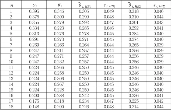
What follows the true values θ_i's refer to the baseball players' actual batting averages for the remainder of the season. Also, θˆ

i, HB1 and θˆ

i, HB2 are denoted by the two different HB estimates of θ_i respectively. The stand errors associated with θˆ

i, HB1 and θˆ

i, HB2 are denoted by s _{i, HB1} and s_{i, HB2} respectively.

It turns out that

( 18σ²)^{- 1}∑

18

1 (y_i- θ_i)²= 0.9345 ( 18σ²)^{- 1}∑

18 1 ( θˆ

i, HB1- θ_i)²= 0.2937 ( 18σ²)^{- 1}∑¹⁸

1 ( θˆ

i, HB2- θ_i)²= 0.3295

The HB estimates serve well as point estimates. The HB1 estimates are slightly better than HB2 estimates overall. But two HB estimates are quite a comparable.

Table 1. The true value, the maximum likelihood estimates and the two HB estimates with standard errors.

n y_i θ_i ˆθ

i, HB1 s_{i, HB1} ˆθ

i, HB2 s_{i, HB2}

1 0.395 0.346 0.305 0.049 0.318 0.046

2 0.375 0.300 0.299 0.048 0.310 0.044

3 0.355 0.279 0.292 0.047 0.301 0.043

4 0.334 0.223 0.285 0.046 0.292 0.041

5 0.313 0.276 0.278 0.045 0.284 0.040

6 0.291 0.273 0.271 0.045 0.274 0.040

7 0.269 0.266 0.264 0.044 0.265 0.039

8 0.247 0.211 0.257 0.044 0.256 0.039

9 0.247 0.271 0.257 0.044 0.256 0.039

10 0.247 0.232 0.257 0.044 0.256 0.039

11 0.224 0.266 0.250 0.045 0.246 0.040

12 0.224 0.258 0.250 0.045 0.246 0.040

13 0.224 0.306 0.250 0.045 0.246 0.040

14 0.224 0.267 0.250 0.045 0.246 0.040

15 0.224 0.228 0.250 0.045 0.246 0.040

16 0.200 0.288 0.242 0.045 0.236 0.041

17 0.175 0.318 0.234 0.047 0.225 0.042

18 0.148 0.200 0.226 0.048 0.214 0.044

(11)

References

1. Datta, G. S. and Ghosh, J. K. (1995). On Priors Providing Frequentist Validity for Bayesian Inference. Biometrika 82, 37-45.

2. Datta, G. S., Ghosh, M. and Mukerjee, R. (2000). Some New Results on Probability Matching Priors. Calcutta Statistical Association Bulletin 50, 179-192.

3. Efron, B. and Morris, C. N. (1975) Data Analysis Using Stein's Estimator and Its Generalizations. Journal of the American Statistical Association 70, 311-319.

4. Ghosh, J. K. (1994). Higher Order Asymptotics. Institute of Mathematical Statistics and American Statistical Association, Hayward, California, USA.

5. Kass, R. E. and Steffey, D. (1989). Approximate Bayesian Inference in Conditionally Independent Hierarchical Models (Parametric Empirical Bayes Models). Journal of the American Statistical Association 84, 717-726.

6. Morris, C. N. (1983). Parametric Empirical Bayes Confidence Intervals. In Scientific Inference, Data Analysis and Robustness, Academic Press, New York, 25-50.

[ received date : Oct. 2004, accepted date : Nov. 2004 ]