pISSN 1229-3008 eISSN 2287-6251
Progress in Superconductivity and Cryogenics
Vol.17, No.2, (2015), pp.31~35 http://dx.doi.org/10.9714/psac.2015.17.2.031
A study on the effect of the condition number in the magnetic field mapping of the Air-Core solenoid
Li Huang and Sangjin Lee
*Uiduk University, Gyeongju, Republic of Korea
(Received 23 February 2015; revised or reviewed 10 June 2015; accepted 11 June 2015)
Abstract
Mapping is a useful tool in the magnetic field analysis and design. In some specific research area, such as the nuclear magnetic resonance (NMR) or the magnetic resonance imaging (MRI), it is important to map the magnetic field in the interesting space with high accuracy. In this paper, an indirect mapping method in the center volume of an air-core solenoid is presented, based on the solution of the Laplace’s equation for the field. Through the mathematical analysis on the mapping calculation, we know that the condition number of the matrix, generated by the measurement points, can greatly affect the error of mapping result. Two different arrangement methods of the measurement points in field mapping are described in this paper: helical cylindrical line (HCL) method and parallel cylindrical line (PCL) method. According to the condition number, the HCL method is recommended to measure the field components using one probe. As a simple example, we mapped the magnetic fields in a MRI main magnet system. Comparing the results in the different methods, it is feasible and convenient to apply the condition number to reduce the error in the field mapping calculation. Finally, some guidelines were presented for the magnetic field mapping in the center volume of the air-core solenoid.
Keywords : Condition number, error of magnetic field mapping, helical cylindrical line
1. INTRODUCTION
In many applications of the magnet, such as the nuclear magnetic resonance (NMR) or the magnetic resonance imaging (MRI), it is important to obtain accurate information about the magnetic fields [1]. In NMR and MRI, normally a map of the magnetic field distribution is needed to guarantee the uniformity of the field in a warm bore volume. The direct way for the magnetic field mapping is to measure the magnetic field at many points in the interesting volume. However, in order to ensure the accuracy of the reconstruction, the number of the measurement points will be very considerable and the measurement time also can be very long [2]. On the contrary, the indirect way uses several measurement points to obtain the expression of the magnetic field. According to the magnetic field satisfying the Laplace’s equation in the source free area, the solution of the Laplace’s equation is used to describe the magnetic field [3]. And the magnetic field mapping becomes to use the measurement data to fit the mathematic equation. Thus, the mapping becomes a powerful tool for adjusting the homogeneity of the magnetic field. But the arrangement of the measurement points in the space greatly affects the mapping results. A suitable choice of the measurement points will lead to a good mapping result.
In this paper, we introduced some basic theorems of the magnetic field mapping in the air-core solenoid and the principle of the condition number in the mapping.
According to the arrangements of the measurement
points, we described two mapping methods: HCL method and PCL method. Using the comparative analysis, the effects of the condition numbers were shown. As a simple example, the two methods were applied to the magnetic field mapping in a MRI main magnet. At last, we proposed several suggestions on how to improve the accuracy of the field mapping in the air-core solenoid.
2. BASIC THEORY OF MAPPING 2.1. Mapping Procedure
The purpose of the mapping is to find the magnetic field distribution in the space. Assume the existence of a magnetic scalar potential 𝑉
𝑚, whose negative gradient gives the magnetic field 𝑩. Due to no current sources in the central volume of the air-core solenoid, the scalar potential 𝑉
𝑚should satisfies the Laplace’s equation,
∇
2𝑉
𝑚= 0.
In the spherical coordinates (𝑟, 𝜃, 𝜑), where 𝑟 is radial distance, 𝜃 is polar angle and 𝜑 is azimuthal angle, the magnetic field in the z-direction, 𝐵
𝑧(𝑟, 𝜃, 𝜑) in the central volume of the solenoid may be expressed by [4]:
∑∑
∞= =
+ +
+
=
0 0
) sin cos
)(
( ) 1 ( )
, , (
n n m
nm nm
nm
z
r r
nn m P u A m B m
B θ ϕ ϕ ϕ
(1) where 𝑃
𝑛𝑚(𝑢) is the set of Legendre polynomials (for m
= 0) and associated Legendre functions (for m > 0) with 𝑢 = cos 𝜃, 𝐴
𝑛𝑚and 𝐵
𝑛𝑚are constants.
* Corresponding author: [email protected]
A study on the effect of the condition number in the magnetic field mapping of the Air-Core solenoid
As shown in (1), if the constants 𝐴
𝑛𝑚and 𝐵
𝑛𝑚are known, the magnetic field 𝐵
𝑧(𝑟, 𝜃, 𝜑) at any point can be calculated through the coordinates of the point. The field mapping is reduced to obtain the constants 𝐴
𝑛𝑚and 𝐵
𝑛𝑚.
In practice, (1) needs to be considered to have finite terms of summation. And the effective cut-off can be found according to the accuracy in the mapping. Assume there are 𝑁 terms needed to sum in (1) and for convenience reasons, (1) is rewritten as matrix form:
X M
B
zm=
zm(2)
where 𝑩
𝑧𝑚is a vector of the z-axis component of the magnetic field at the measurement points, 𝑩
𝑧𝑚= [𝐵
𝑧1𝐵
𝑧2⋯ 𝐵
𝑧𝑁]
𝑇, 𝑿 is a vector of 𝐴
𝑛𝑚and 𝐵
𝑛𝑚in (1), 𝑿 = [𝐴
10𝐴
20𝐴
21𝐵
21⋯]
𝑇, and 𝑴
𝑧𝑚is an 𝑁 × 𝑁 square matrix. The matrix 𝑴
𝑧𝑚can be obtained by the coordinates of the measurement points.
According to (2) and the data from the measurement points, the constants 𝐴
𝑛𝑚and 𝐵
𝑛𝑚can be calculated.
Then the z component of the magnetic field at the any points can be mapped by (1) and the coordinates of these points.
2.2. Condition Number in Mapping
In the solution of the constants 𝐴
𝑛𝑚and 𝐵
𝑛𝑚, the matrix 𝑴
𝑧𝑚is very important for the mapping procedure. Because the form of the matrix 𝑴
𝑧𝑚depends on the coordinates of the measurement points, the errors in the calculation are different when we select different measurement points. Here the condition number is employed to evaluate the error in the calculation.
Assume 𝜹
𝑩𝑧𝑚is the disturbance in 𝑩
𝑧𝑚, and 𝜹
𝑿is the disturbance in 𝑿 due to 𝛿
𝑩𝑧𝑚. According to (2), we can obtain
X
B
M δ
δ
zm=
zm(3)
Take norms of both sides in (3),
zm Bzm
X
M δ
δ ≤
−1(4)
From (2), we also can get, X M
B
zm≤
zm(5) According to (4) and (5), the relative error of 𝑿 can be written as
zm zm
zm
B
zmM δ X M
δ
X≤
−1 B(6)
where ‖𝑴
𝑧𝑚−1‖‖𝑴
𝑧𝑚‖ is defined as the condition number of the matrix 𝑴
𝑧𝑚, 𝑘(𝑴
𝑧𝑚). Obviously, when the condition number is very high, a small disturbance of 𝑩
𝑧𝑚can cause a large of the error in the solution. Hence
we can arrange the suitable measurement points to reduce the condition number 𝑘(𝑴
𝑧𝑚) and obtain a satisfactory mapping result.
3. ARRANGEMENT METHODS 3.1. Two Arrangement Methods in Mapping
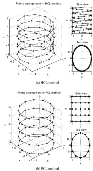
Considering the mapping volume in the center of a solenoid, we can consider two different methods to arrange the measurement points in the mapping as shown in Fig. 1.
According to the trajectory of the measurement points, these methods are named as Helical Cylindrical Line (HCL) method and Parallel Cylindrical Line (PCL) method as shown in Fig. 1. In the HCL method, the measurement points distribute uniformly on a helical cylindrical line, where the radius of the cylindrical surface is R
1, the height of the line is 2H
1and the number of points is N
1. Compared with the HCL method, in the PCL method, the measurement points uniformly distribute on several parallel circles with equal radius R
2, and the distance between the top circle and bottom circle
(a) HCL method
(b) PCL method
Fig. 1. Two arrangement methods of the measurement points in the magnetic field mapping.
-1 0
1 - 1
- 0.5 0 0.5 - 21 - 1 0 1 2
x Points arrangement in HCL method
y
z - 1 0 1- 2
- 1 0 1
2 Side view
x
z
- 1 0 1
- 1 - 0.5 0 0.5
1 Top view
x
y
- 1 0
1 - 1
- 0.5 0 0.5 - 21 - 1 0 1 2
z
Points arrangement in PCL method
y x
- 1 0 1
- 2 - 1 0 1
2 Side view
z
x
- 1 0 1
- 1 - 0.5 0 0.5 1
x
y
Top view
32
Li Huang and Sangjin Lee
is 2H
2. The number of the circles is N
cand the number of points in the circle is N
p.
In the PCL method, the trajectory of the measurement points is the parallel circles instead of the helical line in the HCL method. Thus we can take advantage of multiple probes to measure the field on the cylindrical or spherical surface to reduce the measurement times. On the contrary, it would be better to use only one probe to measure the field in the HCL method. Thus, the structure of the mapping device can be simplified. Especially in the HCL method, the mapping device can be designed to use one probe and one driving motor.
3.2. Experimental Methodology
Assume the measurement points are in the center volume of the solenoid and limited in a cylinder volume, which the maximum radius on the circular surface is a
1. In order to facilitate the discussion, the parameters in the methods are normalized by a
1. According to (2), the number of the measurement points determines the dimension of the matrix ࡹ
௭. Increased dimension of the matrix will lead to an increase in the value of
݇ሺࡹ
௭ሻ. Thus we try to use the same number of points in the methods as much as possible to avoid its effect in the experiments.
In the HCL method, the normalized radius R
1/a
1is less than 1 according to the definition. And the normalized height H
1/a
1assumes less than 2. Definition of the azimuthal angle between two adjacent points is φ
1and the range of φ
1is 0 to π. Using the different parameters, the minimum value of ݇ሺࡹ
௭ሻ is found and plotted as below.
As shown in Fig. 2(b), we can find that the minimum value of ݇ሺࡹ
௭ሻ varies greatly with the azimuthal angle φ
1. In some special cases, such as φ
1=90°, the minimum value of ݇ሺࡹ
௭ሻ becomes infinite.
Compared with φ
1, there is the small influence of R
1/a
1and H
1/a
1on the minimum value of ݇ሺࡹ
௭ሻ according to Fig. 2(a) and Fig. 2(c). The number of points also impacts the value of the condition number. Because it changed the size of ࡹ
௭, the condition number will increase with the number of points used in mapping calculation as shown in Fig. 2(d).
(a) normalized radius (b) azimuthal angle
(c) normalized height (d) number of points
Fig. 2. Influence of parameters in the HCL method.
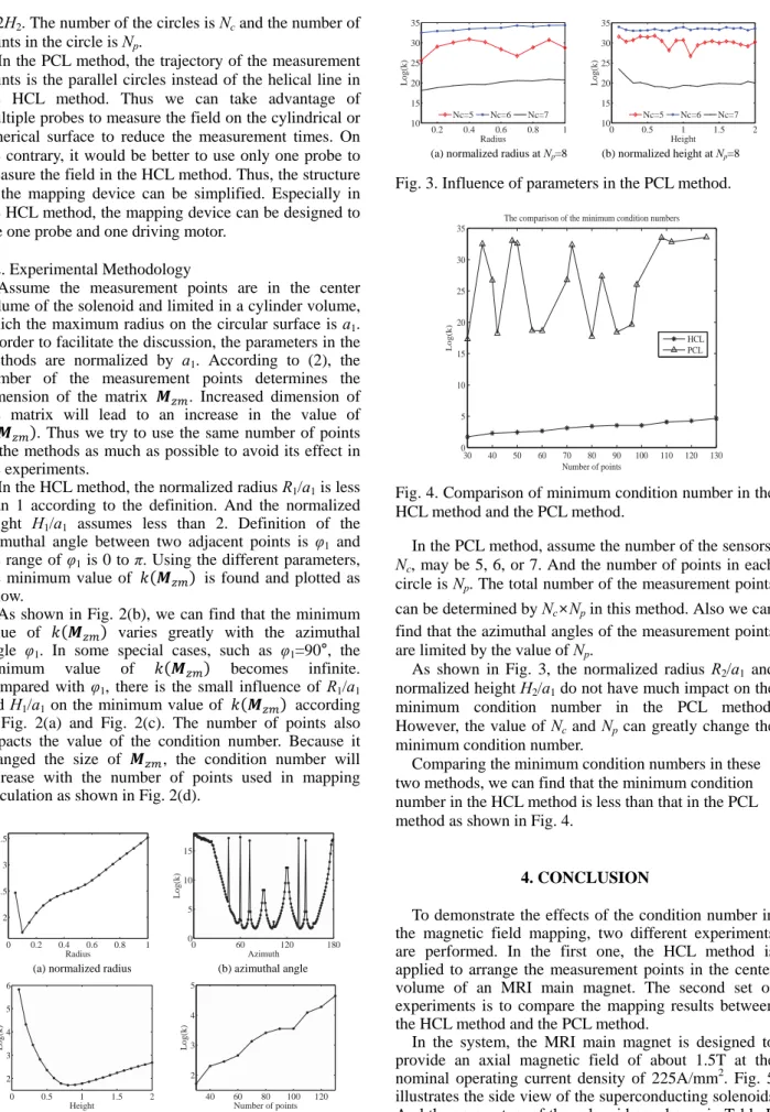
(a) normalized radius at Np=8 (b) normalized height at Np=8
Fig. 3. Influence of parameters in the PCL method.
Fig. 4. Comparison of minimum condition number in the HCL method and the PCL method.
In the PCL method, assume the number of the sensors, N
c, may be 5, 6, or 7. And the number of points in each circle is N
p. The total number of the measurement points can be determined by N
c×N
pin this method. Also we can find that the azimuthal angles of the measurement points are limited by the value of N
p.
As shown in Fig. 3, the normalized radius R
2/a
1and normalized height H
2/a
1do not have much impact on the minimum condition number in the PCL method.
However, the value of N
cand N
pcan greatly change the minimum condition number.
Comparing the minimum condition numbers in these two methods, we can find that the minimum condition number in the HCL method is less than that in the PCL method as shown in Fig. 4.
4. CONCLUSION
To demonstrate the effects of the condition number in the magnetic field mapping, two different experiments are performed. In the first one, the HCL method is applied to arrange the measurement points in the center volume of an MRI main magnet. The second set of experiments is to compare the mapping results between the HCL method and the PCL method.
In the system, the MRI main magnet is designed to provide an axial magnetic field of about 1.5T at the nominal operating current density of 225A/mm
2. Fig. 5 illustrates the side view of the superconducting solenoids.
And the parameters of the solenoid are shown in Table I.
The mapping volume is a sphere in the center of the solenoid. For the sake of the calculation, we used rzBI
0 0.2 0.4 0.6 0.8 1
2 2.5 3 3.5
Radius
Log(k)
0 60 120 180
0 5 10 15
Azimuth
Log(k)
0 0.5 1 1.5 2
2 3 4 5 6
Height
Log(k)
40 60 80 100 120
2 3 4 5
Number of points
Log(k)
0.2 0.4 0.6 0.8 1
10 15 20 25 30 35
Radius
Log(k)
Nc=5 Nc=6 Nc=7
0 0.5 1 1.5 2
10 15 20 25 30 35
Height
Log(k)
Nc=5 Nc=6 Nc=7
30 40 50 60 70 80 90 100 110 120 130
0 5 10 15 20 25 30 35
Number of points
Log(k)
The comparison of the minimum condition numbers
HCL PCL
33
A study on the effect of the condition number in the magnetic field mapping of the Air-Core solenoid
program to obtain the magnetic field generated by the solenoid with high accuracy [5-6].
For the magnetic field mapping in the center volume, the HCL method is firstly applied to arrange the measurement points to obtain the minimum condition number. According to the analysis, we changed the value of the azimuthal angle of measurement points in the HCL method to obtain the different condition number. As shown in Table II, the value of the normalized radius, the normalized height and the number of points are fixed in order to eliminate the influence of the other factors on the mapping.
Fig. 5. Side view of solenoids in the system.
TABLE I PARAMETERS FOR SOLENOID. Coil Width
[mm]
Thickness [mm]
Current Density [A/mm2]
M1 45.2 21 225
M2 106.4 17 225
M3 235.6 21 225
M1’ 45.2 21 225
M2’ 106.4 17 225
M3’ 235.6 21 225
TABLE II
PARAMETERS IN HCL METHOD.
Case 1 2 3
Normalized Radius 0.1 0.1 0.1 Azimuthal Angle 158 43 57 Normalized Height 0.8 0.8 0.8
Number of Point 81 81 81 Logarithm of
Condition Number 3.742228 4.247371 7.466576
(a) on the z-axis (b) on the x-axis
Fig. 6. Error of results in the mapping using the HCL method.
TABLE III
ANALYSIS OF MAPPING RESULTS IN HCL METHOD.
Case 1 2 3
(a) z-axis
SSE 2.14E-5 7.36E-4 2.21E-1 MSE 2.14E-6 7.36E-5 2.21E-2 RMSE 1.46E-3 8.58E-3 1.49E-1 R-square 0.999999 0.999992 0.997781
(b) x-axis
SSE 4.26E-5 7.33E-4 3.10E-1 MSE 4.26E-6 7.33E-5 3.10E-2 RMSE 2.06E-3 8.56E-3 1.76E-1 R-square 0.999998 0.999972 0.987971
TABLE IV PARAMETERS IN PCL METHOD.
Case 4 5 6
Number of Sensors 5 6 7 Normalized Radius 0.1 0.1 0.1 Normalized Height 0.8 0.8 0.8 Number of Point 80 84 84
Logarithm of
Condition Number 18.28831 32.24966 33.82820
(a) on the z-axis (b) on the x-axis
Fig. 7. Error of results in the mapping using the PCL method.
TABLE V
ANALYSIS OF MAPPING RESULTS IN PCL METHOD.
Case 4 5 6
(a) z- axis
SSE 1.97E+2 9.85E+2 - MSE 1.97E+1 9.85E+1 - RMSE 4.44E+0 9.92E+0 - R-square -0.984933 -8.90639 -
(b) x- axis
SSE 6.58E+0 4.75E+2 - MSE 6.58E-1 4.75E+1 - RMSE 8.11E-1 6.89E+0 - R-square 0.744414 -17.4664 -
The logarithm of the error in the mapping results is plotted in Fig. 6 and the sum of squares due to error (SSE), mean squared error (MSE), root mean squared error (RMSE), and coefficient of determination (R- square) are also calculated in Table III. According to Fig.
6 and Table III, we can find that the mapping results become worse when the condition number increases.
Using the PCL method to map the magnetic field, the parameters are selected to close the values in the HCL method and listed in Table IV. The condition numbers in the PCL method are much larger than in the HCL method.
The condition number is 10
3.74in Case 1. However it is almost an increase of 10
15times in Case 4. As shown in Fig. 7 and Table V, the mapping results in the PCL method are worse than the HCL method because the condition number increase. Even in Case 6, there is no result in the magnetic field mapping.
5. CONCLUSION
To map the magnetic field in the center volume of the air-core solenoid, two different arrangement methods of the measurement points are presented. According to the comparison of the mapping results, the condition number of the matrix can greatly affect the error in the mapping results. Generally mapping with a small condition number is better than that with a large condition number.
The mapping results will become unreliable when the condition number in mapping is too large.
0 10 20 30 40 50
-5 -4 -3 -2 -1 0
z [mm]
Log(error) [Gauss]
Case 1 Case 2 Case 3
0 10 20 30 40 50
-5 -4 -3 -2 -1 0
x [mm]
Log(error) [Gauss]
Case 1 Case 2 Case 3
0 10 20 30 40 50
-1 -0.5 0 0.5 1 1.5
z [mm]
Log(error) [Gauss]
Case 4 Case 5 Case 6
0 10 20 30 40 50
-1 -0.5 0 0.5 1 1.5
z [mm]
Log(error) [Gauss]
Case 4 Case 5 Case 6
![TABLE I P ARAMETERS FOR SOLENOID . Coil Width [mm] Thickness [mm] Current Density [A/mm2] M1 45.2 21 225 M2 106.4 17 225 M3 235.6 21 225 M1’ 45.2 21 225 M2’ 106.4 17 225 M3’ 235.6 21 225 TABLE II P ARAMETERS IN HCL METHOD](https://thumb-ap.123doks.com/thumbv2/123dokinfo/5237588.624059/4.892.85.438.308.1164/table-arameters-solenoid-thickness-current-density-arameters-method.webp)
