Comparative Analysis of Two EOQ based Inventory Models

1. Introduction

This paper develops and analyzes two inventory models which extend the classical economic order quantity (EOQ) model. One model uses total cost minimization and the other model uses profit maximization. The extensions of these models to the classical economic order quantity are: (1) For the cost minimization model, the cost per unit is a power function of the order quantity whereas the cost per unit is assumed to be fixed in the EOQ model, (2) For the profit maximization model, we consider the cost per unit and the demand per unit time as a power function of the order quantity and the price per unit respectively, whereas the cost per unit is assumed to be fixed and the demand per unit time is independent of the price per unit in the EOQ model. That is, the profit maximization models consider the cost functions for the cost minimization models with the demand per unit time related to the price per unit, (3) In deriving and

analyzing the optimal solutions, we employ geometric programming (GP) technique as well as derivative based classical first and second order conditions.

One of motivating factors for developing these two models is the need to develop different cost functions and demand functions that better model today’s inventory problem by not having the fixed unit cost and demand independent of the price as the EOQ model does.

The cost minimization model can be applied to companies which focus on the production (lot sizing).

The profit maximization model can be used in functionally centralized firms where production (lot sizing) and pricing (marketing) decisions can be made at the same time. The second is the comparison of the models and the relationship between the optimal solutions that can be determined under certain conditions. By comparing the models, we can derive managerial insights and select an optimal inventory policy.

GP has been very popular in engineering design

Comparative Analysis of Two EOQ based Inventory Models

Hoon Jung

Postal Technology Research Center, Electronics and Telecommunications Research Institute, Deajeon, 305-350

EOQ

기반 재고 모델의 비교 분석

정 훈

In this paper, we compare two EOQ based inventory models under total cost minimization and profit maximization to investigate the difference in the optimal solutions. First of all, optimal solutions for both models through geometric programming (GP) techniques are found considering production (lot sizing) as well as marketing (pricing) decisions. An investigation of the effects of the changes in the optimal solutions according to varied parameters is performed by studying optimality conditions as well as by performing numerical analysis.

We then conduct comparative analysis between the models to show the relationships between the optimal solutions of the models where certain conditions in the cost per unit and the demand per unit time are given.

Several interesting economic implications and managerial insights are observed from this analysis.

Keywords: inventory, geometric programming, EOQ

Corresponding author : Senior Researcher Hoon Jung, Postal Technology Research Center, Electronics and Telecommunications Research Institute, Deajeon, 305-350, Fax : +82-42-860-6508, E-mail : [email protected]

Received May 2004; revision received April 2005; accepted August 2005.

research since its inception in the early 1960s. Even though GP is an excellent method to solve nonlinear problems, the use of GP in inventory models has been relatively infrequent. Kochenberger (1971) was the first to solve the basic EOQ model using GP. In Worrall and Hall (1982), GP techniques were utilized to solve an inventory model with multiple items subject to multiple constraints. Cheng (1989) applied GP to solve modified EOQ models and to perform sensitivity analysis. Lee (1993) also illustrated the usefulness of bounding and sensitivity analysis in the profit maximization model.

There have been numerous publications on EOQ models with fixed cost per unit. However, several papers have relaxed the assumption of the fixed cost per unit for the EOQ models since 1990s. For example, Jung and Klein (2004) and Lee (1993, 1994) assumed the cost per unit as a function of the order quantity.

This assumption means that the production exhibits economies of scale when the order quantity increases.

In addition to cost, Kim and Lee (1998), Lee (1993, 1994), and Lee, Kim, and Cabot (1996) relaxed the fixed demand per unit time and assumed the demand per unit time is a function of the price per unit. That is, the demand per unit time is assumed to be dependent upon the price per unit.

In this paper, we compare the cost minimization model to the profit maximization model and investigate the difference in the optimal solutions. The cost minimization criterion is most appropriate for production departments of economic agents which are provided with fixed budgets and no control over the price of the final product.

In contrast, the profit maximization considers the behavior of economic agents who are both sellers (the price is to be determined) as well as producers of a product. Hence, our comparison means that the monopolistic market of the profit maximization model, where the price is controllable, is compared with the competitive market of the cost minimization model where the price is given by the market. The difference in the optimal order quantity of these models indicates the quantity that is over ordered/under ordered due to the error in estimating the cost function and the price function of the models.

That is, it implies that we use the monopolistic market (competitive market) when the competitive market (monopolistic market) should have been used.

From our comparison, we provide the relationships between the optimal order quantities by comparing our cost functions without computing the optimal solutions.

This means that we can determine optimal inventory policy by estimating the cost functions.

The remainder of this paper is organized as follows.

First, we present assumptions and the two models for

total cost minimization and profit maximization. We then optimally determine the order quantity and the price for our models. In the next section, we obtain the optimality results using the first and second order conditions. That is, the change in the optimal solutions according to varied parameters is analyzed to see the effect on inventory policy. Then, we compare and contrast the cost minimization model and the profit maximization model to gain managerial insights.

Finally, we make concluding remarks and comment on future research areas.

2. Assumptions

We define the following variables and parameters for our models.

P = price per unit (dollar/unit, decision variable for maximization model)

Q = order quantity (units, decision variable for minimization and maximization models) D = demand per unit time (units/unit time) C = cost per unit (dollar/unit)

A = ordering cost (dollar/batch)

i = inventory carrying cost rate (%/unit time) a = scaling constant for D

d = scaling constant for C α = price elasticity of demand δ = quantity discount factor

Three assumptions, which are frequently found in the EOQ literature, are used in this paper: (1) replenishment is instantaneous; (2) no shortage is allowed; (3) the order quantity is ordered in batch.

In addition, we assume that the cost per unit is a power function of the order quantity displaying quantity discounts for the minimization model. That is,

δ

= dQ−

Q

C( ) . For the maximization model, we assume that C(Q)= dQ^−δ and D(P)= aP^−α. D(P)= aP^−α indicates that the demand per unit time is assumed to be a decreasing power function of the price per unit.

3. Models

3.1 Minimization Model

Given the above definitions and assumptions, the total cost per unit time (= TC(Q)) of the minimization model is the sum of the ordering cost per unit time, variable cost per unit time, and inventory holding cost per unit time. Then, we have the following mathemati-

cal formulations from the GP perspective.

Min TC(Q) = AD/Q + C(D, Q)D + iC(Q)Q/2

= ^{ADQ−1+dQ−δD+0 idQ.5 1−δ} (1) The objective function of the minimization model is an unconstrained posynomial with one degree of difficulty. The development of the solution procedure for this model is similar to the work by Cheng (1989, 1991). In the unconstrained posynomial GP problem, the dual variable, wi, provides the weight of ith term of the primal problem over Q by the following equation.

) ( ^*

*

* w d w

U_i = _i (2)

) (w^*

d is the optimal dual objective function and the optimal weights, ^{, *}2^,

* 1 w

w and, w^*3 represent proportions of the setup cost (U1^*), the variable cost (U^*2), and the inventory holding cost (U^*3) to the total cost per unit time, respectively. We then have the following relations for our models.

[ ]^{* 1}

* 1

=ADQ −

U ,^{U*2 =dD}[ ]^{Q* −δ}, ^{U3* =0.5id}[ ]^Q*1−δ (3) The optimal weights can be calculated from the dual problem and the substituted dual problem using GP technology(Cheng (1991) and Jung and Klein (2004)).

Then, the corresponding primal solutions can be obtained from equation (3) (see Appendix).

[ ^{*2 *} ]^1/δ

*

* 1

* AD/(w d(w )) dD/(w d(w ))

Q = =

[

^{( *3 ( *)/(0.5 )}

]

^1/(1−δ)

= w d w id (4)

3.2 Maximization Model

Under the above definitions and assumptions, the profit per unit time (=π^(P,Q)) of the maximization model is the revenue per unit time minus the sum of the above total cost per unit time. Then, we have the following mathematical formulations for the profit per unit time.

Max ^π(P,Q) = PD(P) [AD(P)/Q + C(Q)D(P) + iC(Q)Q/2]

= ^{aP1−α −AaP−αQ−1 −adP−αQ−δ}

−δ

−^{0 idQ.5 1} (5)

The development of the solution procedure for the

maximization model is found in Lee (1993). The objective function, equation (5), is a signomial problem with one degree of difficulty. Although global optimality is not guaranteed for a signomial problem, the profit function can be transformed into a posynomial problem with one additional variable and constraint. This technique was developed by Duffin, Peterson, and Zener (1976). In the constrained posynomial GP problem, the dual feasible solutions,

λ

ωi ^and , provide the weights of the terms in the constraints of transformed primal problem by the following equation.

4 , 3 , 2 , 1 ,

/ =

= i

V_i ω_i λ (6)

∑

∑

= =

=

=

4

1 4

1

and 1 where

i i i

Vi λ ω

These weights represent proportions of the profit (V1), the ordering cost (V2), the variable cost (V3), and the inventory holding cost (V4) to the total revenue. We then have the following relations for our models.

z P a

V₁ = ^{−1 α−1} , ^{V2 =AP−1Q−1},

−δ

=dP−Q

V₃ ¹ , ^{V4 =0.5ia−1dPα−1Q1−δ} (7) From the above equations, the corresponding primal solution can be obtained (see Appendix).

[ ^{−δ 2δ/ 3}]^[1/(1−δ)]

= A dV V

P

[ 2 4/(0.5 3)]^{[1/( −1)]}

= adVV idAV ^α

[ 3/( 2)]^[1/(1−δ)]

= AV dV

Q

[ ]

δ δ δ α

δ

δ

α −

−

− −

−

−











= ¹

1

) 1 /(

) 1 ( 2

) 1 /(

) 1 ( 3 4

5 .

0 id A dV V

aV (8)

The optimal weights are computed from the dual problem and the substituted dual problem, and

*

*and Q

P are calculated from equation (8).

According to the duality theorem of GP, we can obtain π* from the relationship (1/^z*)=^d(ω^*) where π^* = z* = Max z. Therefore, π^*=^1/d(ω^*). Also, _π^* can be obtained from the profit function (5) after

*

*and Q

P are substituted.

4. Optimality Results

4.1 Minimization Model

From the first and second derivatives of the optimal order quantity and the optimal total cost, we investigate the changes in ^Q* and TC^* according to varied parameters, A, i, d, D, and_δ . Since the closed form solutions can not be obtained, we use the implicit function theorem (see e.g., Hildebrand (1976)) with the first and second order conditions.

The first and second order conditions for the global optimality from the total cost function (1) are

0 )

1 2(

1 1

2 − + − =

−

∂ =

∂ ^ADQ₋ δ^dDQ_−−δ δ ^idQ_−δ

Q

TC (9)

δ δ

δ ^{− −}

− + +

∂ =

∂ 3 2

2 2

) 1 (

2ADQ dDQ

Q TC

0 )

1 2 (

1 ₁

>

−

− δ δ idQ^−−δ (10)

First, we investigate the change of the optimal order quantity as the ordering cost A varies. From the first order condition, (9), using the implicit function theorem, we have

[ ]

^{Q AD}

[ ]

^{Q Q}_A ^dD

[ ]

^{Q Q}_A

D ∂

+ ∂

∂ + + ∂

− ^{* −2} 2 ^{*−3 *} δ(1 δ) ^{* −2−δ *}

[ ] ⁰

) 1 2 (

1 _* ^{1 *}

∂ =

− ∂

− ⁻⁻

A Q Q

id ^δ

δ

δ (11)

Equation (11) can be expressed by

[ ]

^{− δ δ}

[ ] [ ]

^{−−δ δ δ}

[ ]

^−−δ

−

−

− +

= +

∂

∂

* 1

* 2

* 3

* 2

*

) 1 2 ( ) 1

1 (

2ADQ dDQ idQ

Q D A

Q

(12) By applying (10) to (12), we obtain the following result.

0

*

∂ >

∂ A Q

(13) From the second derivative of (12), we can also obtain

∂ =

∂

2

* 2

A Q

[ ] [ ] [ ]

[ ]^{* 3} [ ]^{* 2} [ ]^{* 1 2}

* 1

* 2 3 *

*

) 1 ( 2 ) 1

1 ( 2

2 ) 1 )(

2 ( 2

1 2

) 1 2 (



 + + − −



 



 − + − − −

∂

− ∂

−

−

−

−

−

−

−

−

−

−

δ δ

δ δ

δ δ δ

δ

δ δ δ

δ δ δ

Q id Q

dD Q

AD

Q id Q

dD A Q Q D

< 0 (14)

Equation (13) and (14) indicate that the optimal order quantity is an increasing and concave function with respect to the ordering cost A.

For the total cost, we can apply the above procedure and obtain

0

* >

∂

∂ A TC

, ^{2 0}

* 2 <

∂

∂ A TC

(15) The following results for i, d, D, and δ are obtained by similar procedures shown for A.

0 ,

0 ₂

* 2

* >

∂

< ∂

∂

∂

i Q i

Q

, ^{0, 2 0}

* 2

* <

∂

> ∂

∂

∂

i TC i

TC

(16) 0

,

0 ₂

* 2

*

∂ >

< ∂

∂

∂

d Q d

Q

, ^{0, 2 0}

* 2

*

∂ <

> ∂

∂

∂

d TC d

TC

(17) 0

*

∂ >

∂ D Q

(18) 0

* >

∂

∂ δ Q

(19) The above results indicate that any increase (decrease) in A or decrease (increase) in i or d results in a larger (smaller) optimal order quantity, and any increase (decrease) in A, i, or d results in a larger (smaller) optimal total cost.

Any increase in A leads to higher inventory cost and therefore, at the same time, to higher ^Q* and TC^*. If the inventory holding cost, i, which is the part of total cost, increases, total cost increases. In this case, a decision maker will reduce ^Q* to save the expense of storing inventory. The fact that when we increase the scaling constant for C, ^Q*decreases represents that if the cost per unit is increased by scaling constant, ^Q* will be decreased because of economies of scale.

4.2 Maximization Model

For this model, the changes in ^Q*, P^*, and _π^* according to the changes in the parameters, i, a, d, α , and δ are investigated by the computational analysis.

For the experiment, we use the basic parameter values:

A = 50, i = 0.1, a = 500000, f = 5, α = 2.5, and _δ = 0.2. The values of the parameters to analyze with optimal solutions are allowed to vary ±10 %, ±20 %,

±30 %, , ± 90 %, ±100 % for A, i, a, d, ±1 %, ± 2 %, ±3 %, , ±9 %, ±10 % for α, and ±5 %, ± 10 %, ±15 %, , ±45 %, ±50 % for δ .

The computational results for the changes in the optimal solutions according to the changes in the inventory holding cost, the scaling constant for

demand, and the scaling constant for unit cost is shown in <Figure 1>, <Figure 2> and <Figure 3> respectively.

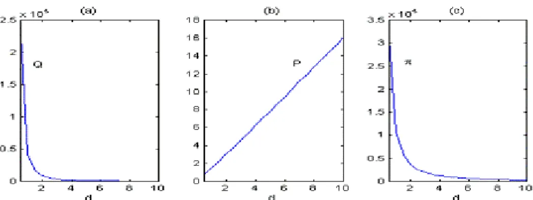
<Figure 1> indicates that any increase (decrease) in inventory holding cost, i, results in a smaller (larger) optimal order quantity, a higher (lower) optimal price, and lower (higher) optimal profit. If the inventory holding cost, i, which is the part of total cost, is increased, total cost will be increased and therefore profit will be reduced. In this case, a decision maker will reduce Q^* to save the expense of storing inventory. From <Figure 2>, we can observe that price

is reduced as a increases since a is a constant for demand and demand is a decreasing function of price.

This results in higher profit and order quantity from the increased demand. <Figure 3> shows that Q^*and π* decrease (_P^* increases) when we increase the scaling constant for C. This represents that if the cost per unit is increased by the scaling constant, ^Q* will be decreased because of economies of scale. Increases in unit cost will lead to higher total cost and price, and hence, lower profit.

Figure 1. Changes in the order quantity (a), the price (b), and the profit (c) with respect to change in the inventory holding cost.

Figure 2. Changes in the order quantity (a), the price (b), and the profit (c) with respect to change in the scaling constant for demand.

Figure 3. Changes in the order quantity (a), the price (b), and the profit (c) with respect to change in the scaling constant for the unit cost.

5. Comparative Analysis

The comparative analysis here is to study the relation- ship between the optimal solutions of the maximization model and the minimization model. The maximization model is a monopolistic market because the model can control both price and demand. However, the minimi- zation model is a competitive market which means that the price is given in the market. Hence, by investiga- ting the difference in the optimal order quantity of the maximization model and the minimization model, we can observe interesting managerial insights. We denote

) and , , ( and ,

, _{c c p p p}

c Q D C Q D

C as the cost per unit,

the order quantity, and the demand per unit time of the minimization model (maximization model), respecti- vely. Also, the asterisk sign means that the value is optimal. We assume that the following parameters are identical for both models: A, i, d, and_δ .

We investigate the error, Qc^*−Q^*p , by comparing Q*’s of the maximization model and the minimization model where certain conditions in the demand per unit time are given. Also, the optimal order quantities of both models are compared where certain conditions in the cost per unit are given. We use the first derivative of the total cost and the profit with respect to the order quantity to compareQ_c^*andQ^*_p.

From the first derivative of the total cost in the minimization model and the first derivative of the profit in the maximization model, and using

α

= p−

p aP

D , we have

[ ] [ ] [ ]^δ

δ δ

−

−

−

− +

*

* 1

* 2

c c c c

c

Q d

Q dD Q

AD

[ ] [ ]

[ ]

^{Q i}

d

Q dD Q

AD

p p p p

p 0.5(1 )

*

* 1

* 2

δ δ

δ

δ

− + =

= ₋

−

−

−

(20)

By manipulating (20), we have the following relationship.

[ ] [ ] [ ]^{* 2} [ ]^{* 1}

* 1

* 2

− +

−

− +

−

+

= +

c c

p p

p c

Q d Q

A

Q d Q

A D D

δ δ

δ δ

(21)

Equation (21) can be used to compare the optimal order quantities in both models for the cases:

,

, ^{* *}

*

*

p c p

c Q Q Q

Q > < and ^Qc*=Q*p under the three

conditions ^{Dc >Dp}, ^{Dc <Dp}, and ^Dc>Dp. If

p

c D

D > , then the right hand side of (21) should be less than 1. This implies ^Qc*<Q*p since [ ]^{Qc* −2+δ} and

[ ]^{Qc* −1} should be greater than [ ]^{Q*p −2+δ} and [ ]^{Q* −p 1}, respectively, to satisfy ^{Dc >Dp} where 0 < δ < 1.

With the similar approach, we can obtain the following property under the three conditions.

Property 1.a If Dc>Dp^,thenQc^*>Q^*p. 1.b If Dc<Dp^,thenQc^* <Q^*p. 1.c If D_c=D_p,thenQ_c^*=Q^*_p.

Property 1.a and 1.b indicate that Dc is maximum and minimum boundary point of ^Dp, respectively.

The difference in the optimal order quantity implies the quantity that is over ordered/under ordered.

Property 1 shows that we can determine optimal inventory policy by estimating ^Dp(we assume that we have previous data of ^Dp) without computing Qc^* and

*

Qp. To estimate the demand function for the model, we first estimate α by applying simple linear regression with previous data for D and P, and then estimate the demand function using α . The estimation of the demand function gives us the relationship between Q_c^* and ^Q*p.

The cost minimization model is appropriate for production departments of economic agents with fixed budgets, and the profit maximization model considers both of production and pricing. Hence, decision maker can apply the above property to choose the better model in certain circumstances whether he wants to focus on both of lot sizing and marketing or he considers only lot sizing. That is, by estimating demand function of maximization model from the previous data, he can adjust the error of the optimal solutions to produce an optimal policy.

From ^d[ ]^{Qc* −δ =Cc andd}[ ]^{Q*p −δ =Cp}, equation (21) becomes

[ ] [ ]

[ ] ^δ [ ] ^δ

δ δ

δ δ

+

− +

−

+

− +

−

+

= + ₁

2 *

*

* 1

* 2

c c c

p p p

p c

Q C Q

A

Q C Q

A D

D (22)

Using (22), we can examine all the cases Qc^*>

,

, ^{* *}

*

p c

p Q Q

Q < and^{Q*c =Q*p} under the three conditions, ,

, _{c p}

p

c C C C

C > < and ^{Cc =Cp}. This yields

Property 2.a. IfCc>Cp^, thenDc<Dpand Qc^*<Q^*p

2.b IfCc<Cp^, then Dc>Dpand Qc^*>Q^*p. 2.c IfCc=Cp^, then Dc=Dpand Q^*c=Q^*p. Property 2 indicates that if Cc and ^Cp can be estimated, the relationship between Cc and ^Cp as well as the relationship between Qc^* and ^Q*p can be analyzed. To estimate the cost function for both models, we first assume that we have previous data for C and Q. Then, for the cost function, C1 =dQ1^−δ ,

−δ

= 2

2 dQ

C , , Cn =dQn^−δ, we can estimate δ by taking the logarithm to transform the cost function into a linear model and then apply simple linear regression.

Hence, the estimation of Cc and ^Cp gives us the relationship betweenQ^*c and ^Q*p as well as maximum and minimum boundary point of ^Dp. Property 2 indicates that we can determine optimal inventory policy from Cc and ^Cp without computing optimal solutions if the difference in the optimal solutions is found. For example, that is, if we know Qc^*>Q^*p (i.e.,

*

Qc is over ordered or ^Q*p is under ordered) from

p

c C

C < , we can increase Cc (or decrease ^Cp) to reduce the error in the optimal order quantity. This adjustment will give us optimal policy for our models.

6. Conclusions

In this paper, we analyzed two EOQ based inventory models under total cost minimization and profit maximization via geometric programming (GP) techniques. We compared and contrasted our models and determined optimal inventory policies without computing solutions. This gave us interesting managerial implications. In addition, we performed optimality analysis to investigate the effects of the changes in the optimal solutions according to the changes in parameters.

The two models we have investigated may provide the basis for numerous further research areas. These models can be a basis for inventory models integrated with quality, setup cost, and process improvement issues (see e.g., Cheng (1989, 1991)). Due to the suitability of GP for dealing with exponential functions, we can apply these to more comprehensive model, where the effects of marketing mix variables

such as advertising and promotion activities on demand are represented by an exponential function.

We can also extend our models to the multi product case where the nonlinear interactions among related products with respect to their demands are taken into account.

Appendix

For the minimization model, we use the following dual problem to solve our problem.

Max d(w)=

[

AD/w1

] [

^w1 dD/w2

] [

^w2 0.5id/w3

]

^w3 (A.1) s. t. ^{w1 +w2 +w3 =1}

0 ) 1

( ₃

2

1− + − =

−w δw δ w (A.2)

0 ,

, _{2 3}

1 w w >

w

There are not enough equations to determine the optimal weights since we have two linear equations and three variables (i.e., under determined). However, we can express the weights, ^{w1andw2,intermsof w3}.

) 1 ( / ) ) 2 ( 1 (

) 1 ( / ) (

3 2

3 1

δ δ

δ δ

−

−

−

=

− +

−

=

w w

w w

(A.3) The normality condition in conjunction with the dual variables being positive yields ⁰<w1^,w2^,w3 <¹. By substituting (A.3) into ⁰<w1^,w2^,w3<¹, we have the following conditions.

) 2 ( / 1 )

2 ( /

1

3 3

δ δ

δ δ

−

<

<

−

<

<

w w

(A.4) From (A.3), if δ ≥1, then w3 ≤δ and

) 2 ( /

3 ≥1 −δ

w to satisfy the positivity condition of the dual variables. But, this does not coincide with (A.4).

Hence, we know that the dual problem is infeasible if

≥1

δ , w3≤δ^, and w3≥^1/(2−δ⁾. Therefore, the positivity condition is

) 2 ( / 1 and , , 1

0<δ < w₃ >δ w₃< −δ (A.5) After combining (A.4) and (A.5), we can obtain the following dual feasibility condition.

Lemma 1. (Dual feasibility condition for minimization model)

If ⁰<δ <^1,0<w1<⁽¹−δ^)/(2−δ^),0<w2<^1, and