논문 2011-48TC-2-2
센서네트워크 상의 노드 밀집지역 간 상호연결을 위한 문제
( Interconnection Problem among the Dense Areas of Nodes in Sensor Networks )
김 준 모**
( Joonmo Kim )
요 약
본 논문은 ad˗hoc 네트워크 또는 센서 네트워크상에서, 주어진 노드들 사이를 상호연결하기 위해 중간노드들을 추가 배치시 키는 형태의 상호연결 문제에 대한 연구이다. 이 문제는 NP˗hard problem으로 변환된다. 네트워크의 노드들은 응용시스템 또 는 지형적인 요인에 의해 일부지역에서는 밀집하여 분포되고, 그 외의 지역에서는 희박하게 분포될 수 있다. 이러한 경우, 노 드들이 밀집한 지역의 상호연결을 무시함으로써, 보다 짧은 실행시간 안에 추가노드들의 최적배치에 근접하도록 하는 방법을 만들 수 있다. 그러나 이러한 경우라 하더라도 여전히 NP˗hard이므로, 동적프로그래밍을 구현함으로써 다항시간 근사전략 (PTAS)을 구성하는 것이 타당하다. 실행결과 등에 대한 분석은 목적함수를 적절하게 정의함으로써 가능해 진다. 목적함수는 노드 밀집지역을 추상화시킴에 의해 발생하게 되는 문제점에 대처할 수 있도록 정의되어야 한다.
Abstract
This paper deals with the interconnection problem in ad˗hoc networks or sensor networks, where relay nodes are deployed additionally to form connections between given nodes. This problem can be reduced to a NP˗hard problem. The nodes of the networks, by applications or geographic factors, can be deployed densely in some areas while sparsely in others. For such a case one can make an approximation scheme, which gives shorter execution time, for the additional node deployments by ignoring the interconnections inside the dense area of nodes. However, the case is still a NP˗hard, so it is proper to establish a polynomial time approximation scheme (PTAS) by implementing a dynamic programming. The analysis can be made possible by an elaboration on making the definition of the objective function. The objective function should be defined to be able to deal with the requirement incurred by the substitution of the dense area with its abstraction.
Keywords : Sensor Networks, Graph Interconnection, NP˗hard Problem, Approximation Algorithm, Steiner Tree Problem
Ⅰ. Introduction
This paper deals with an interconnection problem between nodes in ad˗hoc networks or sensor networks. The nodes of networks, by application or geographic factors, can be deployed densely in some
* 정회원, 단국대학교 컴퓨터학부
(Member, Computer Science & Engineering, Dankook University)
접수일자: 2010년12월23일, 수정완료일: 2011년1월27일
areas while sparsely in others. Over the sparsely deployed network areas, to make the nodes get interconnected with the shortest distance, it is necessary to know the special locations called steiner points[1]: locally interconnecting through which the global interconnection over the network will have the shortest total length. On the other hand, over the densely deployed areas, there is no need to be concerned about the interconnections since it is assumed that the nodes in there are given to be
interconnected. Therefore, by abstracting and simplifying the dense areas, one may construct the approximation scheme effectively that performs the overall interconnections efficiently. As a first thought, one may expect constructing an interconnection scheme by abstracting the dense areas to two dimensional shapes such as circles or rectangles.
However, at this point, one has a problem that it is hard to define or make use of the objective function, which is necessary in analyzing the approximation ratio for the execution results. In analyzing and evaluating the interconnection between nodes, one needs to define and apply the objective function that represents the accumulation of inter node distances over the interconnections. Meanwhile, if the area of two dimensional shape is intermixed in the representation or evaluation of interconnections, it becomes hard to define the objective function, or the evaluation for the execution results becomes complicated or meaningless. So, one needs to devise a gadget that helps to define the objective function. By substituting the dense areas with gadgets, explained in what follows, one is able to omit two dimensional area from the problem instance. After the substitution, one may be able to abstract and define the problem as follows in this section, and construct its approximation scheme in the next sections.
A
gadget
is a two dimensional shape that covers the dense area most appropriately, or it may represent a node of a point. For the purpose of the proof, one should confine a gadget to be a point, a line, a triangle or a rectangle. On the other hand, one may know, from what follows in the next sections, that it can be expanded to be an arbitrary convex polygon. Note that the dense area, which is close to the concave polygon form, can be partitioned into multiple smaller convex polygons. Inside of a gadget is where there is no steiner point, and abstracts the dense area of a network. It can be easily seen that the errors, coming from the abstraction of the dense areas into gadgets, should be reduced into an acceptable level by modifying the gadget into aconvex polygon with more number of sides. The other remaining errors can reasonably be ignored.
Now one may define the interconnection problem for the graph represented by the gadgets as: the problem is to construct the set of interconnection lines that has the minimum total length to interconnect
gadgets
, ⋯. One may see analogous problems in [2~3]. The case that is just one node, which is a point in the abstraction, for all ⋯ is just the Steiner Minimum Tree problem[4], which is NP˗hard. Thus the proposed problem is also NP˗hard[5~6]. For this problem, this paper provides the scheme for constructing its algorithm and its analysis in terms of the execution time and the optimality of the result.
The notations and definitions in the following sections are borrowed from [2~3, 7~8]. Next section is for the definitions in constructing the approximation scheme. Section Ⅲ shows that moving the given problem instance from the real coordinate into the integer one is a necessary and also can be an acceptable modification for the approximation scheme. Section Ⅳ gives component ideas and the main theorem. Section Ⅴ is for the skeleton of the associated dynamic programming and its run time analysis. Section Ⅵ is for the proof of the main theorem, and Section Ⅶ is the conclusion.
Ⅱ. Total Length and Other Definitions
Our objective is to find the interconnection that has the almost minimum sum of the interconnecting edge lengths for the problem instance. For this, first of all, one needs to have definitions and a proposition as follows: is a side (line segment) of the perimeter of a gadget, is the length of , is an optimally interconnecting edges between two gadgets,
is the length of , is an interconnecting edge between two gadgets formed by the approximation,
is the length of , is a graph formed by 's and 's, is for
for
, ℒ is a graph ofall 's, ℒ is for
. Likewise, is a graph formed by 's and 's; , ℒ and ℒ are defined analogously. As well, is a constant, and and are two arbitrarily small constants.It may happen that ℒ comes to be almost zero, and then it becomes meaningless to define the approximation ratio in terms of ℒ. To avoid this situation, one needs to approximate in terms of .
Then the following proposition is in needed.
Proposition 1 Under the reasonable assumption that
for
≤ for
, ˗approximation for implies ˗approximation for the ℒ.Proof:
ℒ for
≤
ℒ for
ℒ ≤ ℒ for
≤ ℒ
ℒ ■
Ⅲ. Shifting into the Integer Coordinates
In order to run the program, the instance of our problem should be shifted into the integer coordinates. The shift will move each end point into the nearest integer position. As well, the steiner
그림 1. 에서 †로의 이동 Fig. 1. Shift from to †.
points, which aids the minimum connection between given nodes, should also lie at the integer positions.
With more definitions that † is on integer coordinate, and
† is on integer coordinate, one may show that the shifts are acceptable.
Proposition 2 ˗approximation over † implies ˗approximation over .
Proof: By the shift and the assumption, one may have the following inequality: † ≤ .
The term is the number of edges of the graph. Note that the maximum number of points for the problem instance is that is the sum of the maximum number, , of points of gadgets and the number, , of steiner points. Considering the tree with nodes, there are edges.
But, may have more edges than the tree due to the shape of gadgets such as triangles or rectangles.
The term 2 is for the maximum length increase by
그림 2. ˗타일링 Fig. 2. ˗tiling.
그림 3. m˗light 그래프 Fig. 3. M˗light graph.
the shift of an edge: each of both ends of an edge can increase its length unit distance at the most.
Likewise, † ≤ , where is an upper bound for the number of edges, supposing the approximated˗graph is a complete network. This condition,
† ≤ ·†, will be shown to be satisfied by the PTAS and then,
≤
≤
≤
where can be chosen appropriately. ■ The term has the key role in this proof, and it can be acquired by setting the unit length of the integer coordinate short enough: gets bigger as the unit of length gets shorter.
Ⅳ. Partitioning, Portals and the Structure Theorem
The first stage of the scheme is to partition the given problem instance so as to form a dynamic programming. A
rectangle
, denoted as
, in partitioning the problem instance is an axis˗aligned rectangle. Thesize
of the rectangle is the length of its longer edge. The bounding box of the problem instance is the smallest rectangle enclosing them. Aline˗separator
, denoted as , of a rectangle is a straight line segment, which is parallel to the rectangle's shorter edge, and which partitions the rectangle into two sub˗rectangles. Each of the sub˗rectangles should occupy at least the area.
For example, if the rectangle's width
is greater than its height, then is any vertical line in the middle
of the rectangle. Now a recursive partition, on which the dynamic programming may run, of a rectangle is defined as follows.Definition 1 ( ˗tiling) A ˗tiling of a rectangle
is a binary tree (hierarchy) of sub˗rectangles of
.
is at the root. If the size of any sub˗rectangle is ≤ , then it's the terminal of the tree. Otherwise, the root contains for
, and has two sub˗trees that are ˗tiling of the two rectangles, into which divides
recursively.Note that the rectangles at depth in the tiling form a partition of the root rectangle. The set of all rectangles at depth is a refinement of this partition obtained by putting through each depth
rectangle of size . The area of any depth rectangle is at most
times the total area. The following proposition is therefore immediate.Proposition 3 If a rectangle has width
and height
, then its ˗tiling has depth at most log
log
.Definition 2 (portals) A portal in a ˗tiling is any point that lies on the edges of rectangles in the tiling. If is any positive integer then a set of portals
is called m˗regular for the tiling if there are exactly equidistant portals on of each rectangle of the tiling. The two crossing points of and
are also portals. In other words, can be divided into equal parts by the portals on it.Definition 3 (m˗light) Let
be a ˗tiling of the bounding box,
be an m˗regular set of portals on
, and ∈
. Then the associated † is m˗light with respect to
if the followings are true: (ⅰ) in each rectangle of tiling
, all 's crosse of that rectangle at most times (ⅱ) each crosses only at portals in
.Theorem (Structure Theorem) The following is true for each . Every set of gadgets in the problem has a ˗approximate
† and an associated ˗tiling
of the bounding box such that the † is m˗light for
, where
log
.
Ⅴ. The Polynomial Time Dynamic Programming (DP)
By Proposition 2 and the proof of the Structure Theorem in the next section,
ʍ˗ can be defined as a
† that has m˗light property and the approximation ratio . One can build ʍ˗
up to the root of the tiling with the DP. The Structure Theorem guarantees the existence of ʍ˗ and its tiling
, where the number of the portals is
log
. By Proposition 3, the depth of
is at most
log . Now, the description for the DP that finds both
and 's for a ʍ˗ comes next in this section. The execution time will be shown to be a polynomial time of · .
The work of the DP is bottom˗up approach, but it is easy to see the procedure from the final stage to the start. The final result of the DP is the rectangle, which is the bounding box for the given problem instance, and which contains the ʍ˗ that can be the almost optimal solution for the problem.
Right before the final rectangle is reached, many combinatorial cases must be checked. All 's that could divide the final rectangle into two sub˗
rectangles according to the ˗tiling are considered one by one as in Fig. 4. Along such a , there are combinations of choices of portals that can be represented by multi˗sets. Then, for each choice of
그림 4. line˗separator를 사용한 분할 Fig. 4. Partitioning with a line˗separator.
그림 5. 포함/제외에 의한 조합
Fig. 5. Combinations from inclusion/exclusion.
and its associated multi˗set of portals, there is one more level of choices for 's. The choices of 's are determined by their inclusions/exclusions within each of the sub˗rectangles as in Fig. 5. For each of the many combinatorial cases, it has its own minimum cost ʍ˗. Such a minimum cost ʍ˗ comes from the concatenation of the two smaller ʍ˗ from each of the sub˗rectangles.
So a rectangle holds as many minimum cost ʍ˗'s as the number of the combinations.
The same observations hold repeatedly in each of the sub˗rectangle for finding its own minimum cost ʍ˗ until the work reaches the bottom most rectangles, where there are limited number of 's, and so the brute˗force algorithm can find the minimum cost ʍ˗ for each of the combinatorial cases inside the smallest rectangle. Out of all the minimum cost ʍ˗'s from the cases of combinations in the root rectangle, the minimum one from them all will be chosen to be the approximated solution for the problem, the final solution.
Now it is to be shown that the number of entries of the lookup table for this DP is a polynomial, and the run time for each of the entries is in a poly time.
An entry can be indexed by the triple: (a) a rectangle, (b) a multi˗set of ≤ portals along the perimeter of the rectangle, and (c) a set of the 's inside the rectangle.
For (a), the number of distinct rectangles is at
most
since the maximum number of points are from the Proof of Proposition 2.For (b), each rectangle has 4 sides, which are parts of the 's of its ancestors. The portals on
are evenly spaced, so they are determined once a is chosen. But the number of choices for a is at most the number of pairs of points, which is
.This accounts for the factor:
. Once the set of portals on the four sides is identified, the number of ways of choosing a multi˗set of size out of them is at most . For (c), if ≤ 's exist in a rectangle, there may exist
possible sets at the most. However, if more than
's pass the of the rectangle, the number of possible sets of the 's inside the rectangle will be artificially set to 1 by using the bridge described in the next section. Hence the upper bound of the size of the lookup table is:
× × ×
,
which is
.
The running time over the lookup table is now to be considered. The bottom level rectangles has limited number of 's of
and so run the brute˗force algorithm for each in time. For each of the upper level rectangles, the minimum value is computed by the comparition operations over the sub˗
rectangles, so the time can be bounded by a polynomial. Therefore, the running time of the DP is upper bounded by × × , which is . Note that the DP is organized so that all the m˗light graphs can be reached. Then, if the existence of ʍ˗ in any chosen rectangle is ensured, the m˗light graph with the minimum length will turn out to be a ʍ˗. The proof of the Structure Theorem in the next section shows the existence of ʍ˗ in a rectangle.
Ⅵ. Proof of the Structure Theorem
The Structure Theorem shows the existence of the ʍ˗ whose difference from
†, which is the mathematical optimality, is arbitrarily small. Once the existence of ʍ˗ is shown, the minimum cost m˗light graph, which will be found by the DP, is naturally a ʍ˗. The proof of the Structure Theorem can be stated as follows. For each rectangle over the ˗tiling of the problem instance, one may choose a that (virtually) crosses with the edges of
† less times than the other 's. Let the points, at which the edges of
† cross with the chosen , be target˗points. Then the ʍ˗whose edges and points cross at the nearest portals to the target˗points will be shown to be within the expected approximation bound.
The analytic sum of the lengths between the target
˗points and their nearest portals, through which the edges of ʍ˗ is passing, may represent the estimation of the length difference between the optimal structure
† and the m˗light structure ʍ˗. The
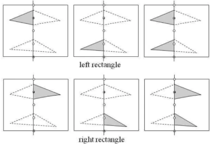
† inside the rectangle can be represented by the minimum possible length estimation, which can be expressed by Lemma 1 that is illustrated in Fig. 6. Let aunit˗band
in a rectangle be the sub˗rectangle with the unit length of width and the height of length
.Lemma 1 When a inside the unit˗band crosses
∈
∪ times with 's or 's, the minimum그림 6. line˗separators를 포함한 6개의 단위 밴드 Fig. 6. Six unit bands with line˗separators.
possible
† in the unit˗band is .Proof: The accumulated length of the line segments, 's or 's, inside the unit˗band gets to be the shortest when all the line segments touch perpendicular to . By the crossings, the minimum cost in the unit˗band is . ■ For each rectangle over the ˗titling, in its middle area, one can be chosen such that the
crosses times with
† while other 's in the same area cross at least times. As a result, the minimum
† in the middle area could be estimated as ·
. Along the chosen , aʍ˗ can be built up. The minimum length m˗
light graphs that has less or equal length than that of ʍ˗ will be found by the DP.
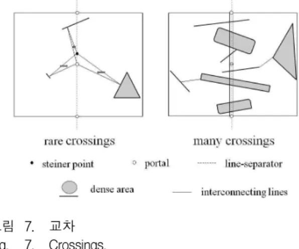
Proof: (Structure Theorem) One needs to figure out how much more length ʍ˗ has than
†. By the number of crossings between
† and a , there are two cases to be considered as in Fig. 7.Case I For a rectangle, there is a , which is crossed ≤ times by
†, where is the minimum number of the crossings that a in the rectangle may have.Case II For a rectangle, all the 's cross with
† more than times.In Case I, the maximum length difference between
그림 7. 교차 Fig. 7. Crossings.
† and ʍ˗ in a rectangle can be
when all the crossing points of ʍ˗ at the portals are steiner points of degree 3, and each of the associated edges increase the length up to
to reach the nearest target˗points. This is due to the properties of steiner tree interconnections[1, 4]. Thus, the ratio of the length difference to
† in the rectangle turns out tobe:
. Now one may let
log
so that the ratio of the length of ʍ˗ to
† is≤
.
In Case II, the estimated minimum
† in the area of a rectangle is
·
since .Let be a bridge inside a sub-rectangle. A bridge is a line segment that lies in parallel with and tightly close to (, but not touching to) the in the rectangle. Note that a rectangle should contain two
's because each of the two sub˗rectangles may have one respectively. The 's, 's and steiner points of a ʍ˗ in one sub˗rectangle will shown to be connected to those in the other sub˗rectangle with the intentional use of 's for the analysis purpose. In fact, a is one of 's. Because the density of the 's in this case is determined to be high, two 's of length
are added to form a ʍ˗, instead of considering the details, which would involve exponential time complexity, of the crossings. Actually, all 's and 's are assumed to be touched with a , instead of passing through portals. Later the two 's are connected with each other through the portal by an infinitesimally short line segment whose lengths can be ignored. So, the ratio of the length difference to the
† in the rectangle is:
·
. As a result, the length
difference from the two cases is at most . Since the tiling has depth of
log , the approximation ratio is
log
log
≤ ■
Ⅶ. Conclusion
The purpose of the scheme is to find the location, called steiner point, so as to form the interconnection that has the shortest total length. One may design a polynomial time algorithm from the scheme. As the algorithm can handle more portals, execution time will increase within a polynomial bound, giving the output with a shorter total length. After having the result of the interconnection algorithm; if there are any two given nodes, which should be connected directly, and which are located far each other beyond the transmission radius of the sensor node, one needs to have another consideration about putting multiple relay nodes between them. This may lead to additional scheme and algorithm with its own analysis, and thus make an independent research later. In implementing the algorithms, the schemes may give the guide for the possible pair of the expected precision of the results and the run time for it, as well as the procedures of the algorithms.
References
[1] E.N. Gilbert and H.O. Pollak, “Steiner minimal trees,” SIAM Journal on Applied Mathematics, Vol. 16, pp.1-29, 1968.
[2] X. Cheng, J.-M. Kim and B. Lu, “A Polynomial Time Approximation Scheme for the Problem of Interconnecting Highways,” Journal of Combinatorial Optimization, Vol 5, issue 3, pp.
327-343, 2001.
[3] DING-ZHU DU, FRANK K. HWANG and
GUOLIANG XUE. “Interconnecting Highways,”
SIAM Discrete Mathematics, Vol. 12, pp.
252-261, 1999.
[4] Z.A. Melzak, “On the problem of Steiner,”
Canadian Mathematics Bulletin, Vol. 4, pp.
143-148, 1961.
[5] Ding-Zhu Du, Ker-I Ko, Theory of Computational Complexity, Wiley Inter-Science 2000.
[6] Michael R. Garey, David S. Johnson, Computers and Intractability A Guide to the Theory of NP-Completeness, Freeman, 1978.
[7] S. Arora, “Polynomial-time approximation schemes for Euclidean TSP and other geometric problems,” Proc. 37th IEEE Symp. on Foundations of Computer Science, pp. 2-12, 1996.
[8] S. Arora, “Nearly linear time approximation schemes for Euclidean TSP and other geometric problems,” Proc. 38th IEEE Symp. on Foundations of Computer Science, pp. 554-563, 1997.
저 자 소 개
김 준 모
(정회원)1989년 서울대학교 컴퓨터공학과 학사
2001년 University of Minnesota 전산학 박사
2002년~2004년 한국정보보호 진흥원 연구원
2004년~현재 단국대학교 컴퓨터학부 부교수
<주관심분야 : Approximations for NP-hard problems>