Development of MATLAB GUI Based Software for Monitoring Ionospheric Disturbances

(1)

1. INTRODUCTION

The satellite signals used in navigations such as Global Positioning System (GPS) and Global Navigation Satellite System (GLONASS) experience signal delays as signals are passed through the ionosphere and troposphere until they reach the users on the ground. The ionospheric delay occurred while passing through the ionosphere is an error that degrades the navigation performance, which should be removed to perform an accurate navigation. It is also used as data to study the ionospheric environment of the earth.

Disturbances occurred in the ionosphere can be detected

ABSTRACT

This study introduces MATLAB Graphical User Interface (GUI)-based software to monitor ionospheric disturbances. This software detects ionospheric disturbances using Global Positioning System (GPS) and Global Navigation Satellite System (GLONASS) measurements, and estimates a location of the disturbance source through the detected disturbance. In addition, this software includes a sky plot making function and frequency analysis function through wavelet transform. To evaluate the performance of the developed software, data of 2011 Tohoku earthquake in Japan were analyzed by using the software. The analysis results verified that the ionospheric disturbances were detected through GPS and GLONASS measurements, and the location of the disturbance source was estimated through the detected disturbance.

Keywords: monitoring software, ionospheric disturbances, epicenter estimation, MATLAB GUI

by analyzing the ionospheric delay of satellite signals. The ionospheric disturbance occurs by events occurred in space such as solar wind as well as natural disasters such as volcano eruptions, earthquakes, and tsunami or events occurred on the ground such as rocket launch or mine explosion (Komjathy et al. 2016). Among them, studies on the detection of the ionospheric disturbance due to earthquakes through the ionospheric delay of GPS measurements have been conducted (Tsugawa et al. 2011, Jin et al. 2015, Song et al.

2018).

Existing studies proposed an algorithm that detected the ionospheric disturbance using GPS measurements, and algorithm that estimated the location of the disturbance source. This study developed a software based on MATLAB Graphical User Interface (GUI) to detect the ionospheric disturbance automatically as well as to estimate the location of the disturbance source by applying GPS and GLONASS measurements to the proposed algorithm in the previous studies.

Since the development of software that monitors the ionospheric disturbance using real-time measurements has a limit, the software in this study aimed at detecting Received Feb 26, 2019 Revised Mar 12, 2019 Accepted Mar 13, 2019

†

Corresponding Author E-mail: [email protected]

Tel: +82-2-880-7395 Fax: +82-2-878-0559

Bu-Gyeom Kim https://orcid.org/0000-0001-7769-1493

Seonho Kang https://orcid.org/0000-0001-6802-105X

Deokhwa Han https://orcid.org/0000-0002-5549-5413

Junesol Song https://orcid.org/0000-0002-3423-2972

Hyoungmin So https://orcid.org/0000-0001-5279-8833

Kap Jin Kim https://orcid.org/0000-0001-7078-2376

Changdon Kee https://orcid.org/0000-0002-8691-7068

(2)

the ionospheric disturbance using post-processing data of already known events. The event information and GPS and GLONASS measurements at the corresponding dates can be entered in the developed software, and the ionospheric disturbance can be detected through input data and the location of the disturbance source can be estimated. A study by Kang et al. (2018) was referred to in the disturbance detection algorithm and a study by Tsai et al. (2011) was referred to in the algorithm that estimated the disturbance source location. In addition, this software includes a function of sky plot production and analysis on disturbance frequency.

In Chapter 2, overall structure of the software and data processing procedure, and analysis techniques used are explained. In Chapter 3, processing results by the software using the actually occurred earthquake data are presented, and its performance is evaluated.

2. MONITORING IONOSPHERIC DISTURBANCES SOFTWARE

2.1 Component of Software

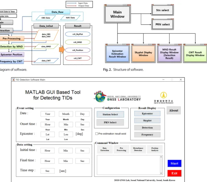
Fig. 1 shows the schematic diagram of the software.

The software detects an ionospheric disturbance utilizing GPS and GLONASS measurements on already occurred events, and estimates the location of the disturbance source accordingly. Thus, post-processing Receiver INdependent Exchange (RINEX) format data are used as an input data.

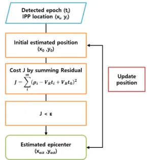
Fig. 2 shows the structure diagram of the developed software. As shown in the figure, two setup screens and four result screens are displayed in the main window. Fig. 3 shows the main window of the software, which is implemented. In the main window, there are two input areas; one is to input information about events to be analyzed, and the other is Fig. 1. Diagram of software.

Fig. 3. Main window of software for surveillance of ionospheric disturbances.

Fig. 2. Structure of software.

(3)

2.2 Algorithm of Software

2.2.1 Algorithm of ionospheric disturbances detection

As mentioned in the introduction, this software detects the ionospheric disturbance using the ionospheric delay of GPS and GLONASS measurements. The ionospheric delay in GPS measurements is calculated through the combination of carrier phase measurements of L1 and L2 frequencies which have a relatively small noise.

1 2

1 1 2 2

1 ( )

1 1

L L

I φ φ I N λ N λ ε

γ γ

= − = + − +

− −

 (1)

Here, Î refers to the ionospheric delay calculated through the measurement combination. Φ refers to the carrier phase measurements, and γ refers to the square of the L1/L2 frequency ratio. I refers to the ionospheric delay at the carrier wave, N refers to the integer ambiguity of each measurement, λ refers to the wavelength of each measurement, and ε refers to the remaining error element. The equation that calculates the ionospheric delay by the combination of carrier measurements is the same as in GLONASS measurement.

However, since frequencies of satellites in GLONASS differ, every satellite in GLONASS has different γ in Eq. (1), which is different from GPS measurement equation.

Kang et al. (2018) proposed a method that detects the ionospheric disturbance by removing the bias component and trend due to the daily change in the ionospheric delay calculated through GPS measurements as well as reducing a noise level. The software in this study detected the ionospheric disturbance using the Minimum Noise Derivative (MND) proposed by Kang et al. (2018). In the MND, the ionospheric delay is assumed as a combination of Gaussian noise and linear trend.

f g v = + (2)

Here, f refers to the ionospheric delay of the measurement

calculated through the combination, g refers to the ionospheric delay of the signal, and v refers to the Gaussian noise. Here, the ionospheric delay at the location which is n epoch away from the i-th epoch can be expressed by Eq.

(3) due to the linear assumption. If Eq. (3) is then arranged by f

_i

', which is a change in the ionospheric delay, (n-1) measurements of change in the ionospheric delay at the i-th epoch can be acquired. Eq. (4) is arranged to calculate the change in the ionospheric delay that produces minimum noise by combining the measurements. As presented in Eq. (4), the change in the ionospheric delay is arranged as a linear combination of the ionospheric delays of N epochs.

The coefficient of the linear combination can be calculated through Eq. (5).

'

1

( 1)

i n i i

f

+ −

= + − f n f (3)

'

1 1 2 2

...

i N N

f = c f c f + + + c f (4)

6 (2( 1) ( 1)) ( 1) ( 1)

c

k

k N

N N N

= − − −

− + (5)

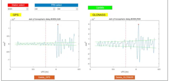
The MND is a technique that calculates a derivative while reducing noise as explained in the above. The ionospheric delay where the MND was applied three times to remove the trend sufficiently was selected as monitoring value of the disturbance detection. Fig. 4 shows the example of the detected disturbance.

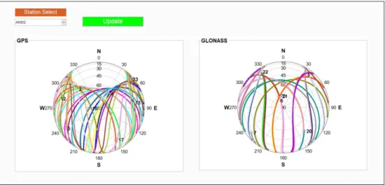
2.2.2 Algorithm of epicenter estimation

In the algorithm of the software that estimates the disturbance source location, a two-dimensional (2D) propagation model, where the disturbance occurred in the disturbance source and reached at 350 km vertically and then propagated in the horizontal direction, was used. Fig.

5 shows the 2D propagation model. This model assumed

Fig. 4. Example of detected ionospheric disturbance.

(4)

that the plane location of the disturbance source was the same between the ground and the ionosphere because the disturbance arrived at the ionosphere vertically from the ground and then propagated horizontally. The data used in the location estimation of the disturbance source were the detection time of the ionospheric disturbance and the Ionospheric Pierce Point (IPP) location at that time. The IPP refers to the location where satellite signals pass through the ionosphere height of 350 km altitude.

Fig. 6 shows an example of the disturbance detection time. As shown in the figure, the disturbance was detected at the first peak epoch in the upper direction, which exceeded the threshold after 10 min of the earthquake. The reason for selecting the region of interest after 10 min of the earthquake was because it took around 10 min for the disturbance occurred on the ground to reach the ionosphere according to the study by Liu et al. (2010). Moreover, the first peak in the upper direction was selected as the disturbance detection time since our data processing results revealed a relatively constant peak occurrence time in the first upper direction

assuming that the estimation error would be the smallest when the same wave was detected from all data used in the epicenter location estimation in the 2D propagation model.

The location at that epoch was designated as IPP latitude and longitude which were defined as the location where GNSS satellite signals pass through the ionosphere height of 350 km altitude.

The distance from the disturbance source to IPP where the disturbance was detected in the 2D propagation model can be expressed as Eq. (6).

(

0

)

i

V t t

R i

ρ = − (6)

Here, ρ

i

refers to the distance from the disturbance source to IPP at the time of disturbance detection, V

R

refers to the propagation velocity of the ionospheric disturbance, t

_i

refers to the disturbance detection time, and t

0

refers to the time taken for the disturbance to arrive at the ionosphere height of 350 km altitude for the first time. The disturbance propagation velocity was set to 3.5 km/s and the time for the disturbance to arrive at the ionosphere was set to 10 min according to the study by Jin et al. (2015). ρ

i

can be calculated through the previously known value and disturbance detection time. However, since the disturbance source location is not known actually, the location cannot be estimated only with ρ

i

. Thus, the disturbance source location is estimated with the algorithm using the cost function.

Fig. 7 shows the schematic diagram of the algorithm that estimates the disturbance source location. For the input data, the disturbance detection time and the latitude and longitude of IPP at that time were used. If the IPP is well distributed Fig. 5. 2D ionospheric disturbance propagation model.

Fig. 7. Algorithm of epicenter estimation.

Fig. 6. Example of detected epoch.

(5)

2.2.3 Algorithm of frequency analysis

This software includes a function to analyze the disturbance frequencies. The reason why the frequency analysis is necessary is to improve the criteria, by which disturbance detection time used as an input data to estimate the location of the disturbance source was selected without any problems. There may be abnormal data of disturbance detection time, which was selected to a suspicious time as noise rather than disturbance if measured data was processed to detect the disturbance automatically in contrast with the case of simulations. Since errors increase if such data were used to estimate the disturbance source location, those abnormal data are required to be removed.

However, abnormal data are difficult to be identified from the ionospheric delay values itself as shown in Fig. 6. Thus, the criteria to classify the abnormal data were improved through the frequency analysis.

Occhipinti et al. (2013) reported that specific frequencies were generated if disturbance occurred in the ionosphere, which were different from the frequencies at normal situations without disturbance. Thus, if there is a large difference between the previously detected disturbance time and a time when the disturbance frequency was generated, it means that this is an abnormal data. As described above, since the frequency analysis results of disturbance should include information on time, the software in this study performed a frequency analysis by applying the wavelet transform to the ionospheric disturbance.

The disturbance frequency of the usual ionospheric delay cannot be verified because the frequency of the trend due to the daily change was the most dominant. To remove this trend, MND may be applied as the same as the above.

However, there was a difference between the frequency of MND processing results and the frequency of original signal. Due to this difference, a high-pass filter was used as much as possible to analyze the disturbance frequency of the original signal. The reason for the use of the high-pass filter was because the trend cycle due to the daily change was

Although the software was designed to enable analyses on various events including earthquakes, the performance of the software in this study was evaluated by analyzing the ionospheric disturbance due to earthquake whose disturbance source location was clear. The analyzed earthquake was Tohoku earthquake (M 9.1) occurred in Japan on March 11 in 2011. The earthquake was regarded as a suitable event to evaluate the software performance because the disturbance detection in the ionosphere was verified by a number of studies by Tsugawa et al. (2011), Tsai et al. (2011), Liu et al. (2011), and Song et al. (2018). For input data, GPS and GLONASS measurements supplied by the reference station in the National Geographic Information Institute (NGII) were employed. The processing results of the software were presented by listing each result windows. Here, the order of the results was made as follows: the sky plot, which was the auxiliary function, was presented first followed by frequency analysis, disturbance detection, and disturbance source location estimation.

3.2 Additional Results

Fig. 8 shows the sky plot of the ANSG reference station.

The sky plot is an auxiliary function because it is not used for detecting disturbance or estimating disturbance source location. However, sky plot can check the distribution of the observable satellites from the reference station.

Fig. 9 shows the frequency analysis results by the software through wavelet transform. It is depicted by using cwt, which is one of the built-in functions in MATLAB. The red line in the graph refers to the earthquake onset time. As shown in the figure, the frequency domain over time can be checked.

In particular, specific frequency domains can be verified after a certain period of time of earthquake.

3.3 Ionospheric Disturbances Detection

The Tohoku earthquake occurred at 5:46:24 (UT). Thus,

(6)

the disturbance was expected to be detected after that time.

The analysis results verified that the disturbance was detected at Pseudo-Random Noise (PRN) 5, 15, 26, and 27 data of GPS and PRN 9 data of GLONASS.

Fig. 10 shows the disturbance detection results verified by the software. It depicts the detection results by PRN of GPS and GLONASS at each reference station. The red line in the graph indicates the earthquake onset time, and the green line indicates the threshold used in the detection. In the graph, the disturbance detection time was marked by a star, which was used to estimate the disturbance source location.

3.4 Epicenter Estimation

The epicenter of the Tohoku earthquake was 38.3 degrees North latitude and 142.4 degrees East longitude according to the seismic survey by the United States Geological Survey (USGS). After setting the estimate location by the USGS to a

true value, the epicenter location estimation was conducted through the location estimation algorithm of the software.

Fig. 11 shows the location estimated results using PRN 5, 15, 26, and 27 data of GPS verified by the software. The epicenter location, estimated epicenter location, and IPP track of the disturbance detected PRN are depicted in the graph. The estimated epicenter location was presented in the upper end and the estimate error was 101.4 km.

This software was implemented to use GPS data as well as GLONASS data. Thus, it can estimate a location by adding GLONASS measurements. Fig. 12 shows the estimated result of the epicenter location when PRN 9 data of GLONASS, where disturbance was detected previously, was added.

The reduction in the estimate error may be expected when GLONASS data is added since the number of used data increased. The estimate error was actually reduced to 91.1 km.

Fig. 8. Sky plot result window.

Fig. 9. Frequency result window.

(7)

4. CONCLUSIONS

This study implemented the ionospheric disturbance monitoring software based on MATLAB GUI. The software included an algorithm to detect disturbance and an algorithm to estimate a disturbance source location through the detected disturbance. It also contained an algorithm that analyzed disturbance frequencies and produced a sky plot as an auxiliary function.

To evaluate the software performance, the Tohoku earthquake occurred in Japan on March 11 in 2011 was analyzed since the earthquake scale was large and well known. The analysis results showed that disturbance was detected in PRN 5, 15, 26, and 27 data of GPS, and when GLONASS measurements were added, disturbance was detected in PRN 9 of GLONASS as well. The estimate error was 101.4 km when only GPS measurements were used to

estimate the epicenter through the detected disturbance whereas the estimate error was 91.1 km when GLONASS measurements were added. When GLONASS measurements were added, the number of available data increased, which was why more accurate estimation could be obtained, and the estimation performance was improved actually. Although the estimate error was not insignificant, this study verified that the ionospheric disturbance could be detected and the disturbance source location could be estimated using the implemented software. If abnormal data are automatically excluded in addition to the improvement on the propagation model for estimation error calculation, the performance of the software will improve further.

ACKNOWLEDGMENTS

This work has been supported by the program ‘Satellite Fig. 10. Detection result window.

Fig. 11. Result of the epicenter estimation (GPS only). Fig. 12. Result of the epicenter estimation (GPS +GLONASS).

(8)

Navigation Augmentation to Improve Navigation Technology’ of Agency for Defense Development, contracted through the SNU-IAMD. This research was supported (in part) by the Institute of Advanced Aerospace Technology at Seoul National University. The Institute of Engineering Research at Seoul National University provided research facilities for this work.

AUTHOR CONTRIBUTIONS

Conceptualization, B.G., S.H. and C.D.; methodology, S.H.

and D.H.; software, B.G.; validation, J.S., H.M., K.J. and C.D.;

formal analysis, B.G.; investigation, B.G.; resources, S.H., D.H.

and J.S.; data curation, B.G. and C.D.; writing—original draft preparation, B.G.; writing—review and editing, J.S. and C.D.;

visualization, B.G.; supervision, C.D.; project administration, C.D.; funding acquisition, H.M. and K.J.

CONFLICTS OF INTEREST

The authors declare no conflict of interest.

REFERENCES

Jin, S., Occhipinti, G., & Jin, R. 2015, GNSS ionospheric seismology: Recent observation evidences and characteristics, Earth-Science Reviews, 147, 54-64.

https://doi.org/10.1016/j.earscirev.2015.05.003

Kang, S., Han, D., Song, J., & Kim, B. 2018, Improving Detection Performance of Ionospheric Disturbances by Optimization of Sequential Measurement Combination, in Proceeding of ISGNSS 2018, November 21-23, 2018, Bali, Indonesia

Komjathy, A., Yang, Y. M., Meng, X., Verkhoglyadova, O., Mannucci, A. J., et al. 2016, Review and perspectives:

Understanding natural-hazards-generated ionospheric perturbations using GPS measurements and coupled modeling, Radio Science, 51, 951-961. https://doi.

org/10.1002/2015RS005910

Liu, J. Y., Chen, C. H., Lin, C. H., Tsai, H. F., Chen, C. H., et al. 2011, Ionospheric Disturbances Triggered by the 11 March 2011 M9.0 Tohoku Earthquake, JGR, 116, A06319. https://doi.org/10.1029/2011JA016761

Liu, J. Y., Tsai, H. F., Lin, C. H., Kamogawa, M., Chen, Y. I., et al. 2010, Coseismic ionospheric disturbances triggered by the Chi-Chi earthquake, JGR, 115, A08303. https://

doi.org/10.1029/2009JA014943

Occhipinti, G., Rolland, L., Lognonne, P., & Watada, S. 2013, From Sumatra 2004 to Tohoku-Oki 2011: The systematic GPS detection of the ionospheric signature induced by tsunamigenic earthquakes, JGR, 118, 3626-3636.

https://doi.org/10.1002/jgra.50322

Song, J., Kang, S., Han, D., Kim, B., & Kee, C. 2018, Real- Time Detection of Ionospheric Disturbances Induced by Earthquake with Detection Window Considering Ionospheric Activity, in Porceeding of the 31st ION GNSS+ 2018, September 24-28, 2018, Miami, Florida, pp.2869-2878. https://doi.org/10.33012/2018.15863 Tsai, H. F., Liu, J. Y., Lin, C. H., & Chen, C. H. 2011, Tracking

the epicenter and the tsunami origin with GPS ionospheric observation, Earth Planets Space, 63, 859- 862. https://doi.org/10.5047/eps.2011.06.024

Tsugawa, T., Saito, A., Otsuka, Y., Nishioka, M., Maruyama, T., et al. 2011, Ionospheric disturbances detected by GPS total electron content observation after the 2011 off the Pacific coast of Tohoku Earthquake, Earth Planets Space, 63, 875-879. https://doi.org/10.5047/

eps.2011.06.035

Bu-Gyeom Kim is a M.S. student of the GNSS Laboratory in the Department of Aerospace Engineering at Seoul National University. He r e c e i v e d B . S d e g r e e i n a e r o s p a c e engineering from the same university. His main research interest is SBAS and ionospheric disturbances by earthquakes.

Seonho Kang is a M.S. student of the GNSS Laboratory in the Department of Aerospace Engineering at Seoul National University. He r e c e i v e d B . S. d e g r e e i n a e r o s p a c e engineering from the same university. His main research interest is ionospheric disturbances by earthquakes.

Deokhwa Han is a postdoctoral researcher of the GNSS Laboratory in the School of Mechanical and Aerospace Engineering at Seoul National University. He received B.S.

and Ph.D. degrees from the same university.

His recent research interests are SBAS and

ionosphere modeling.

(9)

Agency for Defense Development (ADD) in Korea, Republic of. He received B.S. degree in mechanical engineering at Korea Univ.

and M.S. and Ph.D. degree in aerospace engineering at Seoul National University (SNU). He worked in the field of GNSS and pseudolite receiver development including SDR and vector tracking loop algorithm in SNU GNSS laboratory. Since 2011, he's been working for ADD. His research interests are GNSS receiver, anti-jamming/spoofing algorithm, and WADGPS technologies.

Kap Jin Kim is a principal researcher of Agency for Defense Development (ADD) in Korea, Republic of. He received B.S. and M.S.

degree in control and instrumentation engineering at Hanyang University. He worked in the field of Inertial Navigation System(INS) development including initial alignment algorithm in Hanyang University Guidance and Navigation laboratory. Since 2001, he's been working for ADD. His research interests are GNSS and NAVWAR technologies.