Future subsurface drainage in the light of climate change in Daegu, South Korea

Article

Future subsurface drainage in the light of climate change in Daegu, South Korea

Temba Nkomozepi, Sang-Ok Chung ^*

Department of Agricultural Engineering, Kyungpook National University, Daegu, 702-701, Korea

기후변화에 따른 대구지역 지하배수 전망

은코모제피 템바․정상옥 ^*

경북대학교 농업토목공학과 Abstract

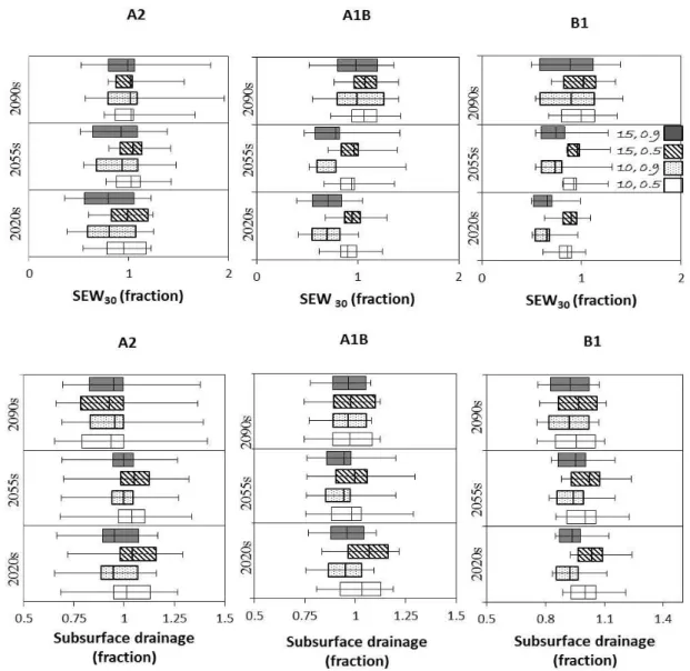
Over the last century, drainage systems have become an integral component of agriculture. Climate observations and experiments using General circulation models suggest an intensification of the hydrologic cycle due to climate change. This study presents hydrologic simulations assessing the potential impact of climate change on subsurface drainage in Daegu, Republic of Korea. Historical and Long Ashton Research Station weather generator perturbed future climate data from 15 general circulation models for a field in Daegu were ran into a water management simulation model, DRAINMOD. The trends and variability in rainfall and Soil Excess Water (SEW

) were assessed from 1960 to 2100. Rainfall amount and intensity were predicted to increase in the future. The predicted annual subsurface drainage flow varied from -35 to 40 % of the baseline value while the SEW

varied from -50 to 100%. The expected increases in subsurface drainage outflow require that more attention be given to soil and water conservation practices.

Keywords：subsurface drainage, climate change, general circulation model, DRAINMOD

Introduction ¹⁾

A well‐designed subsurface drainage system with reasonable drain space and depth contributes to large ratio of desalination and high crop yield (Shao et al. 2012). In the Republic of Korea, subsurface drainage has been implemented in 13% of the wetlands to control water logging and land salinization (Jung et al. 2010). The subsurface drainage project sites include Buyeo, Dongjin and Haman districts among others (Kim and Goo 1977).

The hydrology of fields with single or nonparallel drains may be simulated by determining effective drain spacing by calibration (Skaggs et al. 2012). Most of the existing drainage systems were designed according to the American Society of Agricultural and Biological Engineers (ASABE) scientific criteria and with drain spacing of 7 to15 m and depths of 0.5 m (Jung et al. 2010). Subsurface drainage is a function of local site conditions including climate, soil, cropping system, farming practices, and drainage system (Skaggs et al. 2012a). Approaches to subsurface drainage engineering have assumed the stationarity of rainfall series. Comprehending the response of precipitation to climate change assists in climate change mitigation and

adaptation interventions on subsurface drainage (Coulibaly and Shi 2005).

Analyses of historical data trends have shown evidence of temporal changes in hydro-climatic variables (Jung et al. 2011).

Examination of observed daily precipitation data from the Republic of Korea showed increasing trends in the summer precipitation amount and intensity (Chang and Kwon 2007).

It is widely recognized that in Korea, the impacts of climate change on subsurface drainage will manifest more through changes in extremes than as a result of changes in the mean climate (Xu et al. 2012). Generally, the overall consensus amongst GCM predictions and observations of historical climate data is consistent with monotonic change for temperature (Rogelj et al. 2012).

Difficulties in modelled extreme rainfall result from a lack of enough data to provide a stable estimate of their frequency and intensity. Nevertheless, many studies have shown that the projections from GCMs to be indicative of what we may expect from future rainfall extremes (Fowler et al. 2010). Review of pertinent literature shows that the impacts of climate change

Received: November 7, 2012 / Revised: December 17, 2012 / Accept: December 20, 2012

*

Corresponding Author: Sang-Ok Chung, Tel. 82-53-950-5734, Fax. 82-53-950-6752, Email. [email protected]

©2012 College of Agricultural and Life Science, Kyungpook National University

on sub‐surface drainage in Daegu have not been previously studied.

The objective of this study is to simulate the impact of climate change on the sub surface drainage systems currently installed in vicinity of Daegu.

2)

Study Area

Daegu lies in a basin surrounded by low mountains. The Geumho River flows along Daegu’s northern eastern boundary, emptying in the Nakdong River. The soils in Daegu were identified to be gray shale which consists of 2:1 minerals like illite and vermiculite and were derived from parent material residuum (Um et al. 1993). Land use in Daegu can be classified into water bodies (2%), irrigated crops (17%), forests (57%), grasslands (12%) and urban area (12%) (Lee and Kim 2008).

Fig 1. Map of the study area

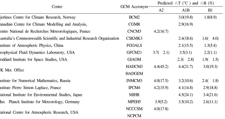
Table 1 GCMs information and predicted changes in temperature and rainfall by the 2090s

Centre GCM Accronym Predicted △T (°C ) and △R (%)

A2 A1B B1

Bjerknes Centre for Climate Research, Norway BCM2 ‐ 3.0(19.8) 1.8(8.9)

Canadian Centre for Climate Modelling and Analysis, CGMR ‐ 2.9(16.9) ‐

Centre National de Recherches Meteorologiques, France CNCM3 4.2(16.7) ‐ ‐

Australia's Commonwealth Scientific and Industrial Research Organization CSKMK3 ‐ 2.4(18.6) 1.6(‐4.0)

Institute of Atmospheric Physics, China FGOALS ‐ 2.1(15.5) 1.3(5.4)

Geophysical Fluid Dynamics Laboratory, USA GFCM21 3.7(‐2.1) 3.5(3.1) 2.2(1.1)

Goddard Institute for Space Studies, USA GIAOM ‐ 2.3(‐2.8) 1.9(‐1.5)

UK Met. Office HADCM3 4.4(45.2) 4.4(21.7) 3.0(19.3)

HADGEM

Institute for Numerical Mathematics, Russia INMCM3 4.0(17.5) 3.2(10.6) 2.4(‐1.8)

Institute Pierre Simon Laplace, France IPCM4 4.2(15.9) 4.1(14.8) 2.9(18.8)

National Institute for Environmental Studies, Japan MIHR ‐ 4.5(24.1) 3.4(21.6) Max‐Planck Institute for Meteorology, Germany MPEH5 3.9(5.2) 3.5(10.2) 2.6(11.1)

National Centre for Atmospheric Research, USA NCCCSM 4.0(17.8) ‐ ‐

NCPCM ‐ ‐ ‐

Daegu's climate is humid subtropical climate with an average annual temperature of 13.7℃, the average temperature in August is the hottest 26.1℃ and the coldest 0.2℃ in January. Average annual rainfall is only 1027.9 mm.

Methods

While we do not attempt to perform a rigorous detection and attribution study, changes in the key parameters with time were investigated using simple statistical methods.

Climate Change Data

Historical data from 1960 to 1990 was extracted from the Korean

Meteorological Administration (KMA) (www.kma.go.kr) and

was adopted as the baseline in this study. Future climate change

scenarios for 2011-2030 (2020s), 2045-2065 (2055s) and

2080-2100 (2090s) and A2, A1B and B1 Special report on

emissions scenarios (SRES) scenarios were generated

stochastically by perturbing the baseline climate in line with

the outputs from a 15 GCMs using LARS-WG (Long Ashton

Research Station stochastic Weather Generator). LARS-WG is

computationally inexpensive and enables the efficient

production of large ensembles of scenarios. The LARS-WG

model simulates precipitation occurrence using two–state, first

order Markov chains: precipitation amounts on wet days using

the gamma distribution; temperature and radiation components

using first–order trivariate autoregression that is conditional on precipitation occurrence (Semenov et al. 1997). Table 1 shows the GCMs used in this study and summarizes the projected annual changes from the baseline in rainfall and ambient temperature across the 15 member GCM ensemble by the 2090s.

3)

Correlation of rainfall to sub surface drainage

The subsurface drainage response of a given soil system is governed by soil type, agricultural management practices, rainfall patterns, topography and subsurface conditions (Singh et al. 1996). The correlations of rainfall to subsurface drainage are investigated here because they can indicate a predictive relationship that can be exploited in simulating the response of drainage systems to climate change.

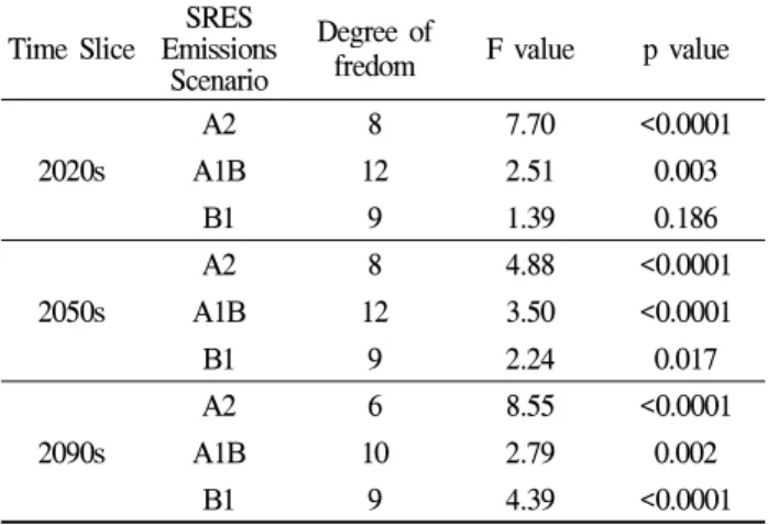
Detection of Rainfall Trends

Analysis of variance (ANOVA) is one of the statistical methods used to determine the differences in different data sets. The single factor ANOVA test was used to determine if there are at least two population means significantly different within each time slice and SRES scenario.

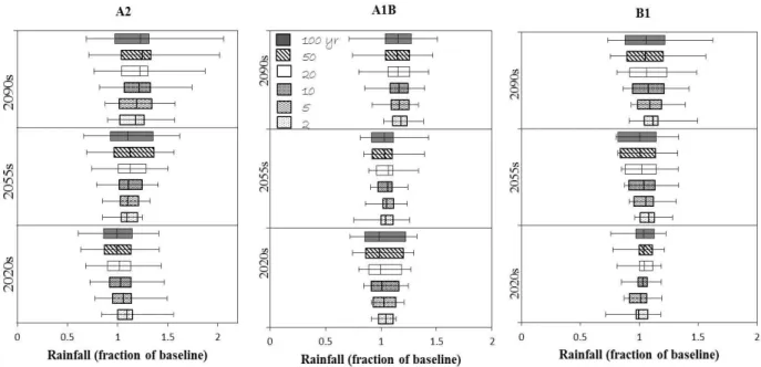
Maximum Rainfall

Annual maxima of daily rainfall for the years 1961-2001 were modelled for five locations in South Korea and there was no evidence suggesting trends in the raw data (Nadaraja and Choi 2007). It is against this background that rainfall return periods were used in order to assess the extreme rainfall. The different rainfall series were fitted to numerous statistical distributions and the most suitable was selected from its ranking by the Kolmogorov-Smirnov and Anderson Darling test. The 3 parameter Gamma distribution (equation 1) was then selected as a statistical model which will capture the difference in behaviour between the baseline and the LARS-WG simulated future scenarios. The shape parameter (α), scale parameter (β) and location parameter (γ) were estimated from the annual daily rainfall maxima series for the respective time slice for the baseline and for each GCM for the future scenarios.

1 ( )/

( ) 1 ( ) ;

( )

f x _a x g ^a e x ^{g b} x g

b a

- - -

= - ³

G (1)

The appropriate 2, 5, 10, 20, 50 and 100 year return period rainfall was calculated from the 3 parameter Gamma survival function.

Mean Rainfall

It has already established that there are no apparent trends in the raw annual mean rainfall (Section 3.2.1) because of the high natural climate variability, therefore the analysis of the trends in mean rainfall were investigated over longer periods of time to deduce the impact of climate change.

Drainage modelling

DRAINMOD is a water management simulation model, which was developed for analysis of soil water movement on a field scale (Skaggs 1980). DRAINMOD is one of the most applied models for the design and evaluation of water management systems (Borin et al. 2000) and was selected for this study.

The model is based on the assumption that lateral water movement occurs mainly in the saturated region, drainage flow is computed by using either the Hooghoudt equation (Eq. 2) or the Kirkham equation (Eq. 3). This approach assumes an elliptical water table shape and is based on the Dupuit- Forchheimer assumptions with corrections for convergence near the drain lines.

2 2

8 kd m _e 4 km

Q L

= +

(2) 4 k t ( b r )

Q GL

p + -

= (3)

where Q is the drainage discharge, d e is the equivalent depth, m is the midpoint water table height above the drain, k is the lateral saturated hydraulic conductivity, L is the distance between drains, t is the surface water depth , b is the depth from drain to the surface, r is drain tube radius. G is a function of L, r, d (the depth from the drain to the impermeable layer) and h (the depth from the surface to the impermeable layer) as given in equation 4 below;

1

1

tan( (2 )(4 ) cosh( / 2 cos( / 2 ) cosh( / 2 ) cos( (2 ) / 2 )

2ln 2 ln

tan( / 4 )

cosh( / 2 ) cos( / 2 ) cosh( / 2 ) cos( (2 ) / 2 )

d r h mL h r h mL h d r h

G r h mL h r h mL h d r h

p p p p p

p p p p p

- ¥

=

é - ù é + - - ù

= ê ë ú û + å ê ë - × + - ú û ₍₄₎

The primary input data required to run DRAINMOD include

weather data, soil data, crop data and drainage system

parameters. The parameters in the above equations are shown

in Fig 2.

Fig 2. Schematics of the soil water movement in DRAINMOD

4)

For soil input data, DRAINMOD requires the relationship between the water table depth and each of upward flux and drainage volume, the soil water characteristic curve, Green- Ampt parameters, lateral saturated hydraulic conductivity. Input data for the model were obtained from the Korean Metereological Administration (www.kma.go.kr), field experiments and estimated from values presented in literature on nearby or within the study areas (Kang et al. 2002, Nkomozepi and Chung, 2011, http://clic.cses.vt.edu/icomanth/06-Asia_

Data.pdf) due to time and cost limitations. Results from Borin et al. (2000) indicated that even very limited input data (texture and porosity of the top 30 cm of soil) gave good predictions.

Typical gridiron subsurface drainage systems were simulated.

A summary of the input drainage design parameters is given in Table 2. In this study the subsurface drainage performance criteria was the Soil Excess Water (SEW 30 ) which is a measure of stress caused by excessive soil water in the top 30 cm.

Table 2 Summary of input drainage design parameters

Parameter Value

Drain depth (cm) 50–110

Drain spacing (cm) 700–1,500

Effective radius of drains (cm) 2

Drainage coefficient (cm/d) 3–5

Actual distance from surface to impermeable layer (cm) 215

Initial water table depth (cm) 50

Results and Discussion Correlation of rainfall to drainage

Climatic variables such as rainfall in particular determine the hydrology of subsurface drained landscapes (Singh et al. 2009).

Fig 3 shows the correlation between baseline rainfall and the simulated subsurface drainage. A strong correlation (R ² = 0.87) exists between rainfall and subsurface drainage. It is evident that subsurface drainage will be sensitive to changes in the amount and intensity of rainfall. The environment is also vulnerable to changes in drainage out flow because subsurface drainage has been identified as a major salt exporter from irrigated areas (Wabba and Christen 2006).

Fig 3. Correlation between baseline rainfall and the simulated subsurface drainage

Trends in rainfall

This study used large rainfall data sets from 15 GCMs. The single ANOVA tests results from each time slice and scenario are shown in Table 3. At least 2 means from the majority of the different rainfall series are established to be significantly (p < 0.01) different at the 0.05 alpha level. The 2020s B1 and 2050s rainfall series were not significantly different. This might be due to the fact that the B1 is the least emissions scenario therefore with little changes to the data they remain close to the baseline values from which all the data is perturbed from.

Table 3 ANOVA tests on rainfall data Time Slice SRES

Emissions Scenario

Degree of

fredom F value p value

2020s

A2 8 7.70 <0.0001

A1B 12 2.51 0.003

B1 9 1.39 0.186

2050s

A2 8 4.88 <0.0001

A1B 12 3.50 <0.0001

B1 9 2.24 0.017

2090s

A2 6 8.55 <0.0001

A1B 10 2.79 0.002

B1 9 4.39 <0.0001

Mean Rainfall

There is general agreement in the predicted mean long term data of the 15 GCMs. Mean rainfall is predicted to drop in the 2020s but gradually increase in the 2055s and 2090s. Table 1 shows some of the predicted changes in rainfall by the 2090s.

A majority of the models predict significant increases in rainfall with the exception of B1, the lower emissions scenario. The harmony between analyses of baseline data and multiple GCM data used herein suggests that the increase in rainfall is consistent with the impacts of climate change rather than mere natural climate variability. ⁵⁾

Maximum daily Rainfall

The 15 GCMs unanimously predicted increasing amounts of maximum daily rainfall corresponding to the given return period as shown in Fig 4. The 50 and 100 year return period maximum daily rainfall was predicted to be as large as double for the A2 scenario as shown in Fig 4. The increase in rainfall intensity could compromise the functionality of the current drainage systems therefore increasing failure risks (Fu et al. in press).

There variability (interquartile range) increases as the return period in increases. The range also generally increases in the future time slices. In this section, we dealt with the maximum daily precipitation amount because of limitations in data availability. It would be more relevant to use 4, 6 or 12 hour maximum rainfall amounts which are more applicable in DRAINMOD.

Fig 4. Predicted future maximum daily rainfall intensity with respect to the baseline for different return periods DRAINMOD SIMULATIONS

Baseline

SEW 30 values are known to be dependent on both surface and subsurface drainage (Skaggs 1980a). Fig 5 shows simulated SEW 30 values for the different combinations of drain spacing and depth. The marginal benefit of drain spacing decreases with increase in the drain depth. It is apparent that in any case wider spacing or deeper depth will decrease the SEW 30 . Other fundamental principles including those of ecology, economics and agronomy also have to be considered in the selection of the suitable drain depth, spacing etc. (Cuenca 1989). For example, selecting shallower drain depth does not deliver major reduction in implementation costs but savings would be more environmental. Salt from deep subsoil is not disturbed, resulting in lower salt loads in the drainage effluent (Van Schilfgaarde 1974). Combinations of 4 drainage systems comprising of 50 and 90 cm drain depth and drain spacing of 10 and 15m were selected to be modelled for the future time slices.

Detailed discussions of drain design specifics are sacrificed for

the sake of other considerations in this paper. Most relevant

to this paper is how the future subsurface drainage will compare

to the baseline in the light of climate change.

Fig 5. Simulated SEW 30 for various drain spacing and depth in the baseline period. ⁶⁾

(50, 70, 90 and 110 refer to drain depth in cm).

Fig 6. Simulated future SEW 30 and subsurface drainage variation with respect to those in baseline period.

Future scenarios

The spread of the simulated subsurface drainage and SEW 30

of the 15 GCMs are given in box and whisker plots shown

in Fig 6. The box represents the interquartile range and the

error bars represent the minima and maxima. The line in the

boxes represents the mean. There is not sufficient evidence

available to conclude a consistent trend in both SEW 30 and

drainage discharge. The simulations do not allude to any

consensus as is evident by the means, large ranges and

interquartile ranges in Fig 6. For the SRES A2 and A1B (with

the exception of 2090s A1B) scenarios, SEW 30 values exhibit

similar skewness patterns, where in the baseline the distributions

are close to symmetric in the 2020s but tend to gravitate towards

left skewness in the future. The B1 however shifts from left

skewness in the 2020s towards a symmetric distribution in the future. Generally, the maximum SEW 30 will decrease from the baseline values with the highest values emanating from the A2 scenario indicating lower drainability in the future. In the most extreme case, the SEW 30 was simulated to have almost doubled by the 2090s. The predicted annual subsurface drainage flow varied from -35 to 40 % of the baseline value while the SEW 30

varied from -50 to 100%. Hydrological consequences of this extent of climate change impact could have a major impact on the design of drainage systems and other hydraulic works in Daegu. Drainage discharge and SEW 30 varied mostly for the B1 and least in the A2 scenario. Drainage values will increase from the baseline values in the 2020s and 2055s but decrease in the 2090s. Despite the changes in mean and maximum daily rainfall being distinctively perceptible, the changes in drainage and SEW possess ambiguity. This could be attributed to the predicted increases in temperature and therefore ET. ⁷⁾ Of the selected drainage systems, the 15m spacing and 0.5m depth (15, 0.5) system showed the highest mean relative changes in SEW 30 and were the most vulnerable to climate change. The 10m spacing and 0.9m depth (10, 0.9) system showed the least relative changes to climate change. The simulation results revealed a weakness of the multi-GCM approach in which the system with the best mean performance has worst extreme. For example the 10, 0.9 system has the least mean relative changes in SEW 30 but also has the highest extreme change (maximum).

It should be noted that the average relative changes should not be interpreted as some measure of consensus or a robust statistic from the 15 GCMs but as a statistical measure of central tendency. While the selection of a single GCM is a major source of uncertainty, the results of multiple GCM simulations are not easily conveyed to end users.

Conclusion

In this paper, the impact of climate change on subsurface drainage system and on the amount and intensity of rainfall in Daegu area has been assessed. It is shown that long term rainfall will decrease in the 2020s and increase in the 2055s and 2090s. The likelihood of occurrence of extreme rainfall events will increase particularly for the 50 and 100 year return period maximum daily rainfall. The drain outflow and SEW 30

were also predicted to increase in the future. The SEW 30 was found to increase by almost 100% in some cases. Hydrological consequences of this extent of climate change impact could have a major impact on the design of drainage systems and other hydraulic works in Daegu area. The assessment of the potential impact of climate change on water systems should

be a part of hydrological research in order to implement the appropriate climate change mitigation and adoption measures.

References

Borin M, Morari F, Bonaiti G, Paasch M, Skaggs RW (2000) Analysis of DRAINMOD performances with different detail of soil input data in the Veneto region of Italy. Agricultural Water Management 42:259-272.

Chang HJ, Kwon WT (2007) Spatial variations of summer precipitation trends in South Korea, 1973-2005. Environmental Research Letters 2(4):045012.

Coulibaly P, Shi X (2005) Identification of the effect of climate change on future design standards of drainage infrastructure in Ontario. Report.http://nickeldistrict.ca/ndca/images/

uploadedfiles/documents/climatechange/finalmtoreportjune 2005rv.pdf

Cuenca, RH, 1989. Irrigation system design.An engineering approach. Prentice Hall. Englewood Cliffs, NJ, USA. ISBN 0-13-506163-6

Fowler HJ, Cooley D, Sain SR, Thurston M (2010) Detecting change in UK extreme precipitation using results from the climateprediction.net BBC climate change experiment.

Extremes 13: 241-267.

Fu X, Tao T, Wang H, Hu T (2012) Risk Assessment of Lake Flooding Considering Propagation of Uncertainty from Rainfall: Case Study. Journal of Hydrologic Engineeringdoi : 10.1061/(ASCE)HE.1943-5584.0000700 (in press) Jung IW, Bae DH, Kim GS (2011) Recent trends of mean

and extreme precipitation in Korea. International Journal of Climatology 31: 359-370.

Jung KY, Yun ES, Park KD, Lee YH, Hwang JB, Park CY, Ramos EP (2010) Effect of subsurface drainage for multiple land use in sloping paddy fields. 19th World Congress of Soil Science, Soil Solutions for a Changing World . Brisbane, Australia

Kang JB, Shin BW, Bang ST (2002) Soil-Water characteristics of unsaturated organic silty soils. Proceedings of the twelfth International offshore and polar Engineering conference , Japan

Kim JG, GooYS (1977) Subsurface drainage for the low wet paddy field(I). Journal of the Korean Society of Agricultural Engineers 19(3):4277-4434.

Lee SH, Kim HD (2008) Effects of regional warming due to urbanization on daytime local circulation in a complex basin of the Daegu Metropolitan Area, Korea. Journal of applied meteorology and climatology 47:1427-1441.

Nadaraja S, Choi DS (2007) Maximum daily rainfall in South

Korea. Journal of Earth System Science 116:311-320.

Nkomozepi T, Chung SO (2011) Estimation of grain size data from the hydraulic conductivity. Agricultural Research Bulletinof Kyungpook National University 29:29-35.

Rogelj J, Meinshausen M, Knutti R (2012) Global warming under old and new scenarios using IPCC climate sensitivity range estimates. Nature Climate Change 2: 248-253.

Semenov MA, Barrow EM (1997) Use of a stochastic weather generator in the development of climate change scenarios.

Climatic Change 35: 397–414.

Shao XH, Hou MM, Chen LH, Chang TT, Wang WN (2012) Evaluation of Subsurface Drainage Design Based on Projection Pursuit. Energy Procedia 16:747-752.

Singh P, Kanwar RS, Johnsen KE, Ahuja LR (1996) Calibration and Evaluation of Subsurface Drainage Component of RZWQM V.2.5. Journal of Environmental Quality 25(1):56-63.

Singh R, Helmers MJ, Kaleita AL, Takle ES (2009) Potential Impact of Climate Change on Subsurface Drainage in Iowa’s Subsurface Drained Landscapes. Journal of irrigation and drainage engineering 135(4): 459-466.

Skaggs RW (1980) DRAINMOD. Reference report. Methods for design and evaluation of drainage-water management systems for soils with high water tables. USDA-SCS, South National Technical Center, Fort Worth, TX, USA Skaggs RW (1980a) Combination surface-subsurface drainage

systems for humid regions. Journal of the Irrigation and Drainage Division 106(4): 265-283.

Skaggs RW, Youssef MA, Chescheir GM (2012) DRAINMOD:

model use, calibration, and validation. Transactions of the ASABE 55(4): 1509-1522.

Skaggs RW, Youssef MA, Chescheir GM (2012a) A DRAINMOD-based method to estimate effects of drainage water management on annual nitrogen loss to surface water.

Transactions of the ASABE 55:799-808.

Um MH, Jung PK, Um KT, Lim HS (1993) Clay mineralogy of the soils derived from gray shale. http://210.101.116.28 /W_kiss3/09400799_pv.pdf

Van Schilfgaarde J (1974) Drainage for agriculture. American Society of Agronomyp .79.

Wahba MAS, Christen EW (2006) Modeling subsurface drainage for salt load management in southeastern Australia.

Irrigation and Drainage Systems 20:267-282.

Xu YP, Zhang X, Tian Y (2012) Impact of climate change on 24-h design rainfall depth estimation in Qiantang River Basin. Hydrological Processes doi: 10.1002/hyp.9210.

8)