Tests for Uniformity : A Comparative Study

2004, Vol. 15, No. 1 pp. 211∼218

Tests for Uniformity : A Comparative Study

Mezbahur Rahman¹⁾ ․ Shuvro Chakrobartty²⁾

Abstract

The subject of assessing whether a data set is from a specific distribution has received a good deal of attention. This topic is critically important for uniform distributions. Several parametric tests are compared.

These tests also can be used in testing randomness of a sample.

Anderson-Darling A² statistic is found to be most powerful.

KeyWords : Approximate Pearson Chi-square statistic, Cramer-Von Misses W2 statistic, Exact Pearson Chi-square statistic, Watson U2 statistic.

1. INTRODUCTION

The subject of assessing whether a data set is from a specific distribution has received a good deal of attention. This topic is critically important for uniform distributions and is different from usual tests for randomness. There are different parametric and nonparametric tests for randomness. A nonparametric textbook such as Daniel(1990) and Gibbons and Chakraborti(2003) would provide extensive references. Marsaglia(2003) and L'Ecuyer and Hellekalek(1998), and the references therein provide a group of tests meant for testing goodness of different random number generators. Here we compare eight different commonly used parametric goodness of fit tests for uniformity through simulation. Let us consider that X₁, X_2,, , X_n be a random sample taken from a Uniform(0,1) distribution. We will first explain all the eight tests. In Section 2 we will provide the simulation results. In Section 3 we will give a brief conclusion based on the simulation results.

1) First Author : Minnesota State University, Mankato, MN 56001, USA E-mail : [email protected]

2) Minnesota State University, Mankato, MN 56001, USA E-mail : [email protected]

1.1. APPROXIMATE χ²_U GOODNESS OF FIT

By grouping the data into g equal groups such that each group has expected frequency of at least five and the number of groups is not too large, we can calculate χ²U goodness of fit statistic as

χ²_U =

Σ

where O_Ui is the observed number of values in the i^th group and E_Ui = n/g is the expected frequency in the i^th group assuming that the sample is from the Uniform(0,1) distribution. The χ²_U statistic will follow approximate Chi-square distribution with g−1 degrees of freedom.

1.2. APPROXIMATE χ²_U GOODNESS OF FIT VIA NORMAL

Box and Muller (1958) showed that if X_{1 and} X₂ are two independent uniform random variables on (0,1), then Z₁ = √

− 2 ln (X₁)sin (2πX₂) and Z₂ = √

− 2 ln (X1)cos (2πX₂) are independent standard normal variates. After using the Box-Muller transformation, we can compute χ²_N statistic as in equation (1). The expected frequencies are computed after computing the cell probabilities using the standard normal table (here we used MATLAB mathematical computational software) and then multiplied by n. It is to be noted that in simulation we have used two independent random samples of size n from Uniform (0,1) distribution to transform to the standard normal but in practice the sample should be divided into two equal groups before applying the Box-Muller transformation. The groups are determined such that the expected frequencies are more than five and are equal.

1.3. EXACT χ²_Z GOODNESS OF FIT VIA NORMAL As we know that the sum of squared standard normal variates follow the Chi-square distribution with n degrees of freedom. So, the test statistic is

χ²_Z =

Σ

n

Z_i² ,

where Z_i's are the standard normal variate after the Box-Muller transformation as in Section 1.2.

1.4. THE CRAMER-VON MISES W² TEST

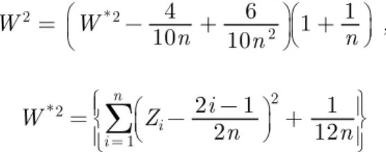
A distribution function test suggested by van Soest (1969), is known as the Cramer-von Mises W² test. The Cramer-von Mises statistic is computed as

W² = ^_





W^*2− ⁴ 

10n + 6 10n²

 

1 + 1 

n , where

W^*2=^





Σ

i = 1 n 

 

Z_i− 2i − 1

2n

2

+ 1 12n

and Z_i= X_{i : n}, the ordered data from the smallest to the largest. The test was modified so that the percentiles are independent of n. In Table 1, the percentiles are displayed. In Table 1, the first line indicates the upper tail probabilities and the second line represents the corresponding quantiles. These are recently recomputed and displayed by D'Agastino and Stephens (1986, p.105).

Table 1 : Upper tail percentiles for cramer-von Mises W² test 0.250 0.150 0.100 0.050 0.025 0.010 0.005 0.001 0.209 0.284 0.347 0.461 0.581 0.743 0.869 1.167

1.5. THE WATSON U² TEST

A distribution function test is suggested by Watson (1961). The Watson U² statistic is computed as

U² = ^_





U^*2− ¹ 

10n + 1 10n²

 

1 + 8 

10n , where

U^{* 2}=^





W^{* 2}−n^_Z− ^1_ 

2

2

,

W^{* 2} and Z_i's are defined above and Z =

Σ

n

Z_i/n. The percentiles are displayed in Table 2. In Table 2, the first line indicates the upper tail probabilities and the second line represents the corresponding quantiles. The test was modified so that the percentiles are independent of n and are given in D'Agastino and Stephens (1986, p.105).

Table 2: Upper tail percentiles for Cramer-von Mises U2 test 0.250 0.150 0.100 0.050 0.025 0.010 0.005 0.001 0.105 0.131 0.152 0.187 0.222 0.268 0.304 0.385

1.6. THE ANDERSON-DARLING A2 TEST

A distribution function test is suggested by Anderson and Darling (1952). The Anderson-Darling A² statistic is computed as

A²=− n − 1

n

Σ

where Z_i's are as above. The percentiles are given in Table 3. In Table 3, the first line indicates the upper tail probabilities and the second line represents the corresponding quantiles. The percentiles are independent of n and are from D'Agastino and Stephens (1986, p.105).

Table 3: Upper tail percentiles for Anderson-Darling A2 test 0.250 0.150 0.100 0.050 0.025 0.010 0.005 0.001 1.248 1.610 1.933 2.492 3.070 3.880 4.500 6.000

1.7. APPROXIMATE χ²_E GOODNESS OF FIT VIA EXPONENTIAL We can easily convert a uniform (0,1) random variate X to a standard exponential variate Y using the transformation Y =− ln (1−X ). Then we can compute the Chi-square statistic as in Section 1.1. Here the expected frequencies are computed by multiplying the group probabilities using the standard exponential CDF(cumulative distribution function). The groups are determined such that the expected frequencies are more than five and are equal.

1.8. EXACT χ²_G GOODNESS OF FIT VIA EXPONENTIAL

We know that 2

Σ

2. Simulation Results

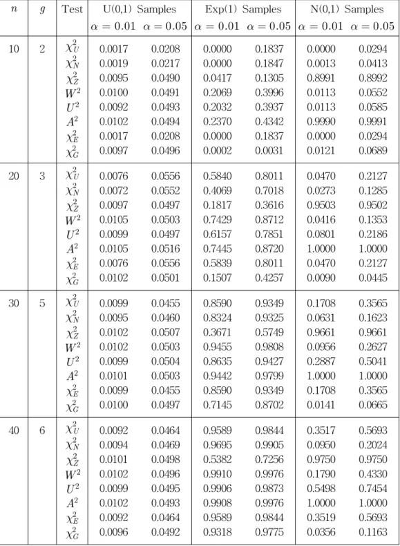
One hundred thousand samples are taken for each of 10, 20, 30, 40, 50, and 100 sample sizes. Then the proportions of rejections are computed for 1% and 5%

levels of significances. Samples are taken from Uniform (0,1) (U(0,1)) to compute the empirical levels of significances to compare with the true levels of significances. Then samples are also taken from standard normal (N(0,1)) distribution as a representative from a symmetric class of distributions and standard exponential (Exp(1)) distribution as a representative from an asymmetric class of distributions to assess the powers of the tests. In the power computations, the samples are transformed such that the range of the data is between 0 and 1 to compute all the statistics mentioned above. The simulation results are given in Table 4.

3. Conclusion

All eight tests are consistently estimating the levels of significances, showing that the distributions under the assumption of uniformity are pretty accurate. In comparison for powers, A² statistic outperform all the tests regardless of the distribution normal or exponential from which samples are taken. χ²Z test has higher power compared to χ²_G test when the samples are from N(0,1) and the role is reversed when the samples are from Exp(1). χ²_U , χ²_N , χ²_E , W², and U² tests have higher powers when the samples are from Exp(1) compared to the samples from N(0,1).

The findings here are consistent with Marsaglia and Zaman (1993) regarding inferiority of Pearsons Chi-square tests and consistent with L'Ecuyer and Hellekalek (1998) regarding superiority of the A² statistic. Note that L'Ecuyer and Hellekalek (1998) did not present any comparative study with Pearson Chi-square tests and with U² and W² tests. Here we also compared between different exact and approximate Pearson Chi-square statistics.

Table 4: Rejection Proportions

n g _Test U(0,1) Samples Exp(1) Samples N(0,1) Samples α = 0.01 α = 0.05 α = 0.01 α = 0.05 α = 0.01 α = 0.05 10 2 χ²_U

χ²N

χ²_Z W²

U² A² χ²_E χ²_G

0.0017 0.0019 0.0095 0.0100 0.0092 0.0102 0.0017 0.0097

0.0208 0.0217 0.0490 0.0491 0.0493 0.0494 0.0208 0.0496

0.0000 0.0000 0.0417 0.2069 0.2032 0.2370 0.0000 0.0002

0.1837 0.1847 0.1305 0.3996 0.3937 0.4342 0.1837 0.0031

0.0000 0.0013 0.8991 0.0113 0.0113 0.9990 0.0000 0.0121

0.0294 0.0413 0.8992 0.0552 0.0585 0.9991 0.0294 0.0689 20 3 χ²_U

χ²_N χ²_Z W²

U² A² χ²_E χ²_G

0.0076 0.0072 0.0097 0.0105 0.0099 0.0105 0.0076 0.0102

0.0556 0.0552 0.0497 0.0503 0.0497 0.0516 0.0556 0.0501

0.5840 0.4069 0.1817 0.7429 0.6157 0.7445 0.5839 0.1507

0.8011 0.7018 0.3616 0.8712 0.7851 0.8720 0.8011 0.4257

0.0470 0.0273 0.9503 0.0416 0.0801 1.0000 0.0470 0.0090

0.2127 0.1285 0.9502 0.1353 0.2186 1.0000 0.2127 0.0445 30 5 χ²_U

χ²_N χ²Z

W² U²

A² χ²_E χ²_G

0.0099 0.0095 0.0102 0.0102 0.0099 0.0101 0.0099 0.0100

0.0455 0.0460 0.0507 0.0503 0.0504 0.0503 0.0455 0.0497

0.8590 0.8324 0.3671 0.9455 0.8635 0.9442 0.8590 0.7145

0.9349 0.9325 0.5749 0.9808 0.9427 0.9799 0.9349 0.8702

0.1708 0.0631 0.9661 0.0956 0.2887 1.0000 0.1708 0.0141

0.3565 0.1623 0.9661 0.2627 0.5041 1.0000 0.3565 0.0665 40 6 χ²_U

χ²_N χ²Z

W² U²

A² χ²_E χ²_G

0.0092 0.0094 0.0101 0.0102 0.0099 0.0102 0.0092 0.0096

0.0464 0.0469 0.0498 0.0496 0.0495 0.0493 0.0464 0.0492

0.9589 0.9695 0.5382 0.9910 0.9906 0.9908 0.9589 0.9318

0.9844 0.9905 0.7256 0.9976 0.9873 0.9976 0.9844 0.9775

0.3517 0.0950 0.9750 0.1790 0.5498 1.0000 0.3519 0.0356

0.5693 0.2024 0.9750 0.4330 0.7454 1.0000 0.5693 0.1163

Table 4 (Continued): Rejection Proportions

n g _Test U(0,1) Samples Exp(1) Samples N(0,1) Samples α = 0.01 α = 0.05 α = 0.01 α = 0.05 α = 0.01 α = 0.05 30 5 χ²_U

χ²_N χ²_Z W²

U² A² χ²_E χ²_G

0.0110 0.0097 0.0105 0.0101 0.0097 0.0108 0.0110 0.0101

0.0462 0.0457 0.0510 0.0495 0.0484 0.0506 0.0462 0.0504

0.9872 0.9943 0.6704 0.9985 0.9901 0.9985 0.9872 0.9865

0.9958 0.9986 0.8212 0.9998 0.9974 0.9998 0.9958 0.9965

0.5145 0.1446 0.9803 0.2962 0.7522 1.0000 0.5145 0.0696

0.7105 0.2790 0.9803 0.6051 0.8842 1.0000 0.7105 0.1751 40 6 χ²_U

χ²_N χ²Z

W² U²

A² χ²_E χ²_G

0.0103 0.0106 0.0101 0.0102 0.0100 0.0105 0.0103 0.0104

0.0503 0.0494 0.0500 0.0507 0.0498 0.0510 0.0503 0.0508

1.0000 1.0000 0.9370 1.0000 1.0000 1.0000 1.0000 1.0000

1.0000 1.0000 0.9727 1.0000 1.0000 1.0000 1.0000 1.0000

0.9629 0.4273 0.9897 0.8930 0.9967 1.0000 0.9629 0.2862

0.9890 0.6212 0.9897 0.9834 0.9992 1.0000 0.9890 0.4365

4. Bibliography

1. T.W. Anderson and D.A. Darling (1952). Asymptotic theory of certain goodness-of-fit criteria based on stochastic processes, Annals of Mathematical Statistics, 23, 193-212.

2. G.E.P. Box and M.E. Muller (1958). A note on the generation of random normal deviates. Annals of Mathematical Statistics, 29, 610-611.

3. R.B. D'Agostino and M.A. Stephens (Eds.) (1986). Goodness-of-Fit Techniques, Marcel Dekker, New York.

4. W.W. Daniel (1990). Applied Nonparametric Statistics, Second Edition, Duxbury Thomson Learning, Pacific Grove, CA.

5. J.D. Gibbons and S. Chakraborti (2003). Nonparametric Statistical inference, Marcel Dekker, Inc., New York.

6. P. L'Ecuyer and P. Hellekalek (1998). Random Number Generators:

Selection Criteria and Testing, in Random and Quasi-Random Point sets, Lecture Notes in Statistics, no. 138, Springer, 223-266.

7. G. Marsaglia and A. Zaman (1993). Monkey tests for random number

generators, Computers and Mathematics with Applications, 26(9), 1-10.

8. G. Marsaglia (2003). Random Number Generators. Journal of Modern Applied Statistical Methods, 2(1), 2-13.

9. J. van Soest (1969). Some goodness of fit tests for the exponential distribution, Statistica Neerlandica, 23, 41-51.

10. G.S. Watson (1961). Goodness-of-fit tests on a circle, Biometrika, 48, 109-114.

[ received date : Nov. 2003, accepted date : Jan. 2004 ]