I. Without Consideration of Water Quality
LEE, Sunhoon··MACHIDA, Isao*··IMOTO, Yukari Graduate School of Science and Technology, Chiba University
Japan Science and Technology Corporation*
(Manuscript received 9 June 2003; accepted 4 July 2003)
상관우물들이 분포하는 화산섬 집수역에 대한 지하수 양수능의 평가 I. 水質을 고려하지 않은 경우
善勳·町田 功*·井本 由香利
千 大學自然科學硏究科, 日本科學技術振興事業團*
(2003년 6월 9일 접수, 2003년 7월 4일 승인)
요 약
본 연구는 値解析을 이용하여 상관우물들의 분포를 갖는 집수역에서 수질을 고려하지 않
은 상태의 지하수양수능을 평가하는 것을 목적으로 한다. 연구지역은 日本의 미야께지마(三 島)이며, 미야께지마는 최근에 이르기까지 火山噴火가 계속되고 있는 화산섬으로 水文地質學的 으로 매우 복잡한 구조를 갖고 있다. 각각의 우물들에 대한 양수능은 個別양수에 의해서 구해 진 IMY(i,t)로써 추정되었으며, 全 연구지역의 양수능은 同時양수에 의해서 구해진SSMY(i,t)로 써 추정되었다. 이러한 결과들은 미야께지마와 같은 화산섬에서 用水공급을 위한 계획의 수립 에 있어서 확실한 공급원의 확보에 이용될 수 있다.
동시양수의 경우, 우물 5와 6에서의 양수는 타이로이께(大 池)부근에 존재하던 지하수가 연 구지역의 내부에 까지 침투하는 것에 대한 障害우물로써 작용했다. 그러므로, 본 연구는 質的,
的 측면에서 용수공급을 위한 지하수의 最適 관리방법으로써 동시양수를 제안한다.
주요어 : groundwater pumping capacity, interrelated wells, individual withdrawal, simultaneous withdrawal, and barrier well
Corresponding Author: Sunhoon Lee, Lab. of Landscape Engineering, Faculty of Horticulture, Chiba University, 648, Matsudo, Matsudo-shi, Chiba, 271-851, Japan Tel & Fax: 81-47-308-8911 E-mail: [email protected]
I. Introduction
To secure the stable sources of water use for human activities is an important problem in Miyake Island, Japan. Most of young volcanic islands generally have little permanent surface runoffs regardless of having abundant precipita- tion. The major causes might be in the very steep slopes from its center to coastlines and the thick volcanic surface deposits with high permeability.
While the former brings about very rapid dis- charge of a part of precipitation through intermit- tent surface runoff into sea, the latter causes the infiltration of the other part of precipitation into underground. Even in young volcanic islands, the existence of groundwater could be found.
It is very difficult to find out the distribution and catchment area of groundwater with a high quality and abundant quantity in a young vol- canic island, because not only the topographical
features of the thick volcanic surface deposits often have a very poor agreement with their underlying layers but also they have remarkable local differences with respect to hydro-geological properties. In the use of groundwater as the source of water use, also, the withdrawal of groundwater from wells is necessary and this should results in; the interference of pumping yields by interrelation between wells and the spread of contaminants from the wells or sources with low quality. In order to solve these prob- lems, it is required to evaluate the pumping yields without and with consideration of water quality using numerical simulation. Pinder and Bredehoeft (1968) used the digital computer for aquifer evaluation. Pinder and Frind (1972) described the application of Galerkin’s procedure to aquifer analysis. Pricket (1975) and Bachmat et al. (1978) used numerical models for evaluating the quantity of regional groundwater. Orlob and
Abstract
The purpose of this paper is to evaluate the groundwater pumping capacity at a catchment area containing interrelated wells without considering their qualities by using numerical simulation in Miyake Island, young volcanic island with very complicated hydro-geological formations. The groundwater pumping capacities of each well and over entire study area were estimated as the IMY(i,t) by individual withdrawals and the SSMY(t) by simultaneous withdrawals. These results can be used to secure a sure source for taking a plan for supplying water use in young volcanic island as Miyake Island.
In simultaneous withdrawals, the withdrawals from well no. 5 and 6 should have the roles as the barrier wells against the intrusion of the groundwater of the part adjacent to Tairo Pond into the inner part of study area. Therefore, it can be suggested to adopt the simultaneous withdrawals as the optimal approach of groundwater management for supplying water use with respect to quantity and quality.
Key words : groundwater pumping capacity, interrelated wells, individual withdrawal, simultaneous withdrawal, and barrier well
Woods (1967) considered the management of water quality in irrigation systems. However, it was never mentioned to evaluate the pumping yields of interrelated wells without and with con- sideration of water quality using numerical simu- lation in order to secure a sure source for taking a plan for supplying water use in the young vol- canic island as Miyake Island.
The purpose of this paper is to evaluate the groundwater pumping capacity at a catchment area containing interrelated wells without consid- eration of water quality using numerical simula- tion in the young volcanic island with very com- plicated hydro-geological formations. This result can be used to secure a sure source for taking a plan for supplying water use in the young vol- canic island. The evaluation of groundwater pumping capacity with consideration of water quality will be subsequently discussed.
II. Study Area
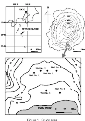
This study was accomplished at the deposits with a light slope and the area of about 0.2 km2 between pond and steep rock slope within a small basin (Figure 1). The pond is called ‘Tairo Pond’ and is located at the center of a catchment area with a distinct basin type. The basin is the most important source for water use in Miyake Island. Also, it was reported to be the crater formed by the volcanic eruption 2500 years ago (Tsukui and Suzuki, 1998). Miyake Island is about 180 km south of Tokyo, Japan and its geo- logical formation is mainly composed of the com- plicate alternations of basalt and volcanic deposits by several volcanic activities with the interval of about 20 years.
The hydraulic conductivities around wells were obtained by pumping test, and the result is shown in Table 1.
III. Theory
The formulation of the equation describing groundwater flow in horizontal two dimensions can be written:
Figure 1. Study area.
Table 1. The groundwater and pumping limited heads at wells and the hydraulic conductivities around wells.
(Kx )+ (Ky )= Ss (1)
where h is hydraulic head in m, Kxand Ky are the components of saturated hydraulic conductiv- ity in the x and y coordinate directions in m/sec, Ssis specific storage in m-1, and t is time in sec.
In order to apply Eq. (1) into the study area of Figure 1, the appropriate boundary and initial conditions are required.
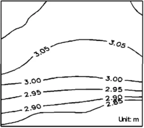
The initial condition, h(x, y, 0) was given by the measured groundwater and pond water heads during February to April 2002, h0(x, y), and the result is shown as the groundwater heads in Table 1 and the distribution of equipo- tential lines in Figure 2. Thus, the initial condi- tion for Eq. (1) is:
h(x, y, 0) = h0(x, y) for t = 0 in G (2) where G denotes the entire flow domain.
The boundary condition of this study area is separated into two parts. The one part, W1is the borderline between Tairo pond and study area and this was treated as Dirichlet boundary condi- tion with a constant head, that is, the initial head of Tairo pond. The other part, W2is the border-
line between steep rock slope and study area.
This part is given as Neumann boundary condi- tion with no flow. Thus, the boundary conditions for Eq. (1) are:
h(x, y, t) = h0(x, y) for t > 0 in W1 (3a)
_ (Kx n_x+ Ky n_y)= qn(t) for t > 0 in W2 (3b) where n_
xand n_
yare unit vectors in the x and y directions and qnis the flux normal to the bound- ary. Water flux at any point in the flow region is given by:
qx= _ Kx (4a)
qy= _ Ky (4b)
where qx and qyare the components of flux in the x and y directions.
This analysis used the linear quardrilateral ele- ments as Figure 3. Its linear shape functions can be defined as:
Ni= (1 + e1 ie)(1 + hih) (5)
4
∂h
∂y
∂h
∂x
∂h
∂y
∂h
∂x
∂h
∂t
∂h
∂y
∂
∂y
∂h
∂t
∂
∂x
Figure 2. The distribution of equipotential lines in initial condition.
Figure 3. Placements of nodes and linear quardrilateral elements for applying Galerkin finite element method into study area.
= (1 + hih) |e = 0,h = 0= (6a)
= (1 + eie) |e = 0,h = 0= (6b)
where e and h are local coordinates and the val- ues of ei and hi are given by Huyakorn and Pinder (1983).
Applying initial and boundary conditions, Eq.
(1) was formulated into the local matrices of 4×4 size by the Galerkin finite element method with the linear quadrilateral elements of 4 nodes.
Then, the local matrices were assembled into the global matrix as:
([C] + wDt[K]){h}t+Dt= ([C] - (1 - w)Dt[K])
{h}t + Dt((1 - w){F}t + w{F}t+Dt) (7)
where [C], [K], {h}, and {F} called the global matrices of capacitance, conductance, head, and specific flow, respectively, w is the relaxation fac- tor, and Dt and t + Dt are the time steps of pre- sent and next, respectively.
The simulator was coded by using the Microsoft Fortran language.
IV. Methods
The evaluation of pumping capacity was accomplished through the use of the pumping rates obtained by individually and simultaneously withdrawing from six wells within the study area.
The withdrawals from wells were carried out by numerical simulation. In individual withdrawals, the pumping rate required for initial head to attain at pumping limited head during a pump- ing time was individually obtained at each well.
This pumping rate will be referred to as ‘IMR’
hereinafter. In simultaneous withdrawals, the pumping rates required for initial head to attain
at pumping limited head during a pumping time were simultaneously obtained at all wells. They will be referred to as ‘SMR’ hereinafter. The mul- tiplications of IMR and SMR by pumping times, t, become the individual and simultaneous dura- tion maximum pumping that will be referred to as ‘IMY’ and ‘SMY’ hereinafter, respectively. The pumping times adopted in both withdrawals were 6, 12, 24, 48, 72, 144, and 288 hours. Also, the changes of IMY and SMY with pumping time were summarized as the approximate expressions for IMY and SMY with pumping time, IMY(i,t) and SMY(i,t), in which i and t indicate well num- ber and pumping time, respectively. Furthermore, the sum of SMY(i,t) at all wells was given as SSMY(t). Therefore, while IMR and SMR or IMY(i,t) and SMY(i,t) mean the duration maxi- mum pumping rate or yield at each well without and with considering the interrelation between wells, SSMT(t) indicates the duration maximum pumping yield over entire study area.
In withdrawing due to numerical simulations, the heads of nodes were obtained. Using these values, the distributions of equipotential lines on over-all study area were produced out. They gave the important information for describing the behavior of groundwater on individual and simultaneous withdrawals from wells and taking a plan for the optimal management in withdraw- ing groundwater.
V. Results and Discussion
1. Evaluation of pumping capacity by individual withdrawals
At each well, the IMP required for the initial hi
4
∂Ni
∂h hi
4
∂Ni
∂h
ei 4
∂Ni
∂e ei
4
∂Ni
∂e
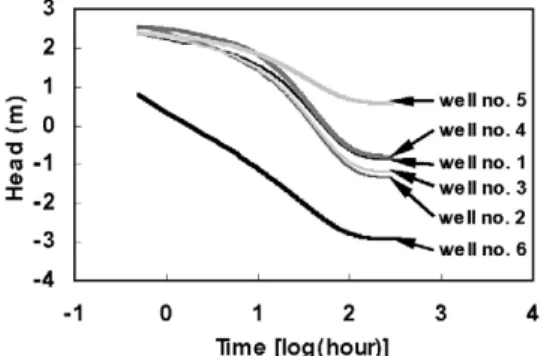
head to attain at the pumping limited head dur- ing the pumping times of 6, 12, 24, 48, 72, 144, and 288 hours was obtained by numerical simula- tion with trial and error. Figure 4 shows the head changes occurred by applying the IMP’s corre- sponding to pumping durations, 6, 12, 24, 48, 72, 144, and 288 hours into well no. 6. Here, the curves of 72, 144, and 288 hours were one anoth- er superimposed. The similarity in these head changes can be acquired in the case that their
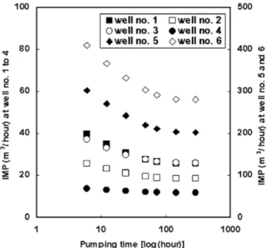
pumping rates approach a constant value under steady state. This fact can be confirmed from very small differences between the values of the last three plots at each well in Figure 5, also.
Because the changes of IMP’s with pumping times relations in Figure 5 show very severe curvilinear trends, it is impossible to summarize them into a exact expression. This difficulty can be overcome by multiplying IMP by pumping time, namely obtaining IMY. The relations between IMY’s and pumping times at wells were found to be linear in Figure 6. Summarizing them, the approximate expression for IMY, IMY(i,t), can be obtained in general form as:
IMY(i,t) = ait + bi (8)
where aiand bithe slope and intercept in the approximate expression for IMY at well i, respec- tively. The values of aiand bi at each well are given in Table 2 and the coefficients of determi- nation, R2, in all cases were greater than 0.999.
The application of Eq. (8) is allowable between 6 and 288 hours.
Figure 5. Changes of IMPs with pumping times at wells.
Figure 6. Relations between IMYs and pumping times at wells. The lines indicate approximate expressions, IMY(i,t), and the coefficients of determination, R2, in all cases were more than 0.999.
Figure 4. Head changes occurred by individually applying the IMPs of pumping times, 6, 12, 24, 48, 72, 144, and 288 hours at well no. 6. The curves of 72, 144, and 288 hours are one another superimposed.
It should be noted that the values of bi in Table 2 are greater than zero. It might be natural that IMP or IMY becomes zero at t = 0. The cause is in adopting the Dirichlet boundary condition with the assumption of a constant head at the borderline between Tairo Pond and study area.
This assumption is resulted from the fact that the withdrawals from wells have no effect on the head of Tairo Pond, since the area of Tairo Pond is very larger than that of study area. In the case having a remarkable head drop with withdrawal, it might be desirable for obtaining the exact solu- tion to adopt the procedure of Lee (2002) that the loss due to head drop and the inflow through borderline are converged by iteration.
Because IMY(i,t) indicates the maximum pumping capacity of respective wells as the func- tion of pumping time without considering the interrelation between wells, it is useful in deter- mining the details related with the pump installa- tion as pump capacity, electric capacity, magni- tude of reservoir or pipe, etc.
2. Evaluation of pumping yield by simultaneous withdrawals
The computations of SMP and SMY(i,t) were accomplished by the similar procedures such as
the cases of IMP and IMY(i,t). Since in the former not only the complicated interrelations between wells but also the heads of the six wells with various hydraulic conductivities, initial heads, pumping limited heads, and distances to two dif- ferent boundary conditions must be simultane- ously attained at pumping limited heads with the smaller error than 10-5, the estimation of SMP through numerical simulation requires an enor- mous computation time.
Figure 7 shows the head changes occurred by simultaneously applying the SMP’s of 288 hours into wells. All curves except for that of well no. 6 have S shapes. The main cause is considered that the horizontal spreading of depression cone due to withdrawal at well no. 6 obstructs them at the other wells. It should be noted that similarly to the cases of IMP (Figure 5) the SMP’s of well no.
6, also, were the largest (Figure 8) even though the hydraulic conductivity of well no. 5 is the largest (Table 1). This means that pumping limit- ed head is an important parameter in determining pumping rate as well as hydraulic conductivity.
The relations between SMY’s and pumping times at wells were shown in Figure 9. The lines Table 2. The values of the aw, bw, cw, and dw for the
approximate equations obtained by individual and simultaneous withdrawals.
Figure 7. Head changes occurred by simultaneously applying the SMPs of 288 hours into all wells.
indicate approximate expressions, SMY(i,t), and the R2in all cases were higher than 0.999. The SMY(i,t) can be expressed in the general form as:
SMY(i,t) = cit + di (9)
where ciand diare the slope and intercept in the approximate expression for SMY with the pump- ing duration t at well i, respectively. The values of ci and di in Eq. (9) were given in Table 2.
Therefore, the sum of the SMY(i,t) in Eq. (9), SSMY(t), can be obtained by:
SSMY(t) = SMY(i,t) = + (10)
The lower and upper limits of pumping time, t, in applying Eq. (10) are 6 and 288 hours.
Because SSMY(t) means the duration maxi- mum pumping yield over entire study area, the evaluation on pumping capacity of a catchment area with interrelated wells must be discussed by this parameter. This can be used to estimate the supply capacity of a catchment area as a source for water use.
3. Behavior of groundwater due to individual and simultaneous withdrawals
The withdrawal of groundwater at a point within catchment area has some effects on behav- ior of groundwater. The effects can be found by the changes of the distribution of equipotential lines occurred due to withdrawal. Figure 10 shows the distributions of equipotential lines obtained by individually applying the IMY’s of 288 hours into wells. In all cases, it clearly appears that the hydraulic gradients were formed with very steep slopes from Tairo Pond toward the inner part of study area as well as the respec- tive pumping wells. This means that groundwa- ter moves from Tairo Pond toward the inner part of study area at high rate. If the part adjacent to Tairo Pond were highly concentrated, the rapid spread of the contaminants of the part adjacent to Tairo Pond into the inner part of study area by individual withdrawals could not escape.
Figure 11 shows the distributions of equipoten-
6
tSdi
i=1 6
tSci
i=1
S6 i=1
Figure 8. Changes of SMPs with pumping times at wells.
Figure 9. Relations between SMYs and pumping times at wells. The lines indicate approximate expressions, SMY(i,t) and the R2in all cases were more than 0.999.
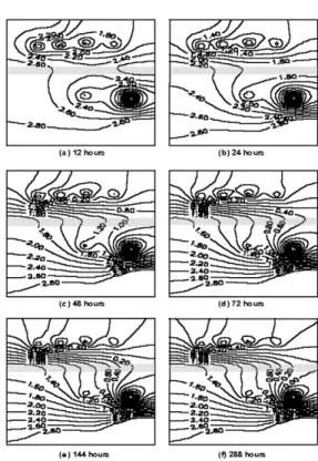
tial lines obtained by simultaneously applying the SMY’s of 12, 24, 48, 72, 144, and 288 hours into all wells. The shadow parts in (a) to (f) indicate the ridge parts of equipotential lines between the alignment of well no. 1 to 4 and that of well no. 5 and 6. Since the heads in these ridge parts have higher than them in the alignments of well no. 1 to 4 and of well no. 5 and 6, they should have the role for preventing the spread of the groundwater of the part adjacent to Tairo Pond into the inner part of study area by simultaneous withdrawals.
Therefore, it is desirable to adopt the simulta- neous withdrawals as the optimal management for supplying water use with respect to its quan- tity and quality. The more detailed considerations for controlling the quality of groundwater by
simultaneous withdrawals will be discussed in the subsequent report.
VI. Conclusion
We evaluated the groundwater pumping capaci- ty at a catchment area containing interrelated wells without consideration of water quality in Miyake Island, a young volcanic island with very compli- cated hydro-geological formations. All parameters obtained by Galerkin horizontal 2-dimensional tran- sient simulator. The withdrawals from wells were individually and simultaneously accomplished.
Figure 10. Distributions of equipotential lines obtained by individually applying the IMYs of 288 hours into wells.
Figure 11. Distributions of equipotential lines obtained by simultaneously applying the SMYs of 12, 24, 48, 72, 144, and 288 hours into all wells. The shadow parts in (a) to (f) indicate the ridge part of equipotential lines between the alignment of well no. 1 to 4 and that of well no. 5 and 6.
The groundwater pumping capacity of each well was estimated as the IMY(i,t) by individual withdrawal. The duration maximum pumping rate, IMP, of each well can be easily obtained by dividing IMY(i,t) by the pumping time. They are useful in determining the details related with the pump installation as pump capacity, electric capacity, magnitude of reservoir or pipe, etc.
The groundwater pumping capacity over the entire study area was estimated as the SSMY(t) by simultaneous withdrawals. The pumping rate of each well correspondent to SSMY(t) can be easily obtained by dividing SMY(i,t) by the pumping time, where the sum of SMY(i,t) becomes SSMY(t). Using SSMY(t), the exact esti- mation of the supply capacity of a catchment area as a source for water use should be possible.
The groundwater behavior resulted from indi- vidual and simultaneous withdrawals was given by the distributions of equipotential lines. While individual withdrawal brought about the rapid movement of the groundwater of the part adja- cent to Tairo Pond into the inner part of study area, in simultaneous withdrawals the movement of the groundwater of the part adjacent to Tairo Pond was interrupted by the occurrence of the ridge parts of equipotential lines between the alignment of well no. 1 to 4 and that of well no.
5 and 6. In simultaneous withdrawals, the with- drawals from well no. 5 and 6 should have the roles as the barriers for the intrusion of the groundwater of the part adjacent to Tairo Pond into the inner part of study area. Therefore, it can be suggested to adopt the simultaneous with- drawals as an approach of the optimal manage- ment of groundwater for supplying water use with respect to quantity and quality.
References
Bachmat, Y., B. Andrews, D. Holtz, and S. Sebastian, 1978, Utilization of numerical groundwater models for water resource management, Report No. EPA-600/8-78-012, Robert S. Kerr Environmental Research Laboratory, Office of Research and Development, U.S. Environmental Protection Agency, Ada, OK 74820.
Huyakorn, P. S. and G. F. Pinder, 1983, Computational methods in subsurface flow, Academic Press, New York, N. Y.
Istok, J., 1989, Groundwater modeling by the finite element method, American Geophysical Union, Water Resources Monograph 13.
Lee, S. H., 2001, Consideration on the validity and physical meaning of parameters in sorptivity expression, Unpublished Ph.D. thesis, Chiba University, Japan.
Orlob, G. T. and P. C. Woods, 1967, Water-quality management in irrigation systems, Journal of the irrigation and drainage division, American society of civil engineers, 93, 49-66.
Pinder, G. F. and E. O. Frind, 1972, Application of Galerkin’s procedure to aquifer analysis, Water Resources Reserch, 8, 108-120.
Pinder, G. F. and J. D. Bredehoeft, 1968, Application of the digital computer for aquifer evaluation, Water Resources Research, 4, 1069-1093.
Pricket, T. A., 1975, Modeling techniques for groundwater evaluation. In: Advances in Hydroscience, 10, Academic Press, New York, 1-143.
Tsukui, M. and Y. Suzuki, 1998, Eruptive history of Miyakejima Volcanic during the last 7000 years, Kazan, 4, 149-166.
최종원고채택 03. 07. 08