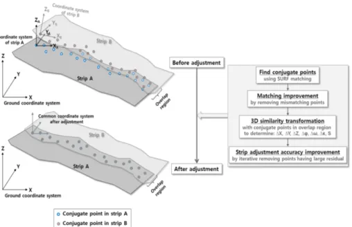
Improvement Scheme of Airborne LiDAR Strip Adjustment
15
0
0
전체 글
(2)
(3)
(4)
(5)
(6)
(7)
(8)
(9)
(10)
(11)
(13)
(14)
(15)
수치
+4
관련 문서
