ISSN 1229-2427 (Print) ISSN 2288-646X (Online) http://dx.doi.org/10.7843/kgs.2014.30.11.17 한국지반공학회논문집 제30권 11호 2014년 11월 pp. 17 ~ 23
JOURNAL OF THE KOREAN GEOTECHNICAL SOCIETY Vol.30, No.11, November 2014 pp. 17 ~ 23
지표면 에너지 수지 이론을 이용한 도로노면온도예측을 위한 예단 모델 개발
The Prognostic Model for the Prediction of the Road Surface Temperature by Using the Surface Energy Balance Theory
송 동 웅1 Song, Dong-Woong
Abstract
In this study, the prognostic model for the prediction of the road surface temperature is developed using the surface energy balance theory. This model not only has a detailed micro meteorological physical attribute but also is able to accurately represent each surface energy budget. To verify the performance, the developed model output was compared with the German Weather Service (DWD)’s Energy Balance Model (EBM) output, which is based on the energy budget balance theory, and the observations. The simulated results by using both models are very similar to each other and are compatible with the observed data.
요 지
본 연구는 지표면 에너지 수지 이론을 이용한 도로노면온도예측을 위한 예단 모델을 개발하기 위한 것으로, 개발된 모델은 지표면 에너지 수지를 정확하게 표현함으로서 매우 복잡한 미기상학적 물리 과정을 표현할 수 있다. 모델의 성능을 검증하기 위하여 독일 기상청의 모델과 비교 실험을 하였으며, 독일의 관측자료 그리고 한국 기상청의 도로기 상 관측 시스템의 관측자료를 이용하여 비교 검증하였다. 비교 결과 독일의 모델 결과와 매우 유사한 결과를 나타냈으 며, 각 관측 자료값들과 잘 일치하였다.
Keywords : Prognostic model, Road surface temperature, Surface energy balance, Micro-meteorological physics
1. Introduction
The thought of surface energy balance has been exten- sively applied for various purposes especially in micro- meteorological analysis of phenomena relating to management of the Earth' resources. Carson (1982) has given a com- prehensive review of land-surface and the atmospheric boundary schemes used in many general circulation models
with an emphasis on surface processes. Schmugge and Humes (1995) applied the surface energy balance model to monitor land surface fluxes. Many studies used Bowen ratio between sensible and latent heat fluxes to estimate the evapolation rate through surface energy balance equation (Brutsaert, 1982; Gutierres et al., 1994). Other papers deal with specific topics in more details, including Zhihao et al. (2002), Du et al. (2013), Lagos et al. (2011), Senay
1 정회원, Member, Prof., Dept. of Environmental Engrg., Sangji Univ., Tel: +82-33-730-0442, Fax: +82-33-730-0442, [email protected]
* 본 논문에 대한 토의를 원하는 회원은 2015년 5월 31일까지 그 내용을 학회로 보내주시기 바랍니다. 저자의 검토 내용과 함께 논문집에 게재하여 드립니다.
Copyright © 2014 by the Korean Geotechnical Society
This is an Open-Access article distributed under the terms of the Creative Commons Attribution Non-Commercial License (http://creativecommons.org/licenses/by-nc/3.0) which permits unrestricted non-commercial use, distribution, and reproduction in any medium, provided the original work is properly cited.
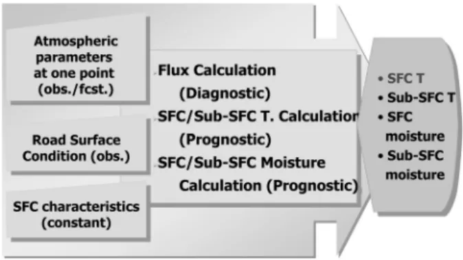
Fig. 1. Overview of schematic process of the developed model
et al. (2010), Sato (2009).
The inclusion of soil surface and road condition is very important in an attempt to improve a land surface parameterization for use in different scale atmospheric models.
The major meteorological factors determining the road condition, such as freezing temperature and micro- meteorological variables, are affected by the road surface temperature. Also topographic features can affect thermally driven road conditions, either directly, by causing changes in the wind direction (Atkinson, 1981) or indirectly, by inducing significant variations in the road surface tem- perature. But under the condition of the wide flat road or bridge, topographical features on the road condition are not significant.
Except for the topographical perturbations, the road-air energy budget exchange has also been found to significantly affect not only the local ground heat budget and but also the surface temperature distribution (Segal et al., 1989;
Betchtold, 1991).
It is evident that the reliable prediction of the road surface temperature, such as determining the freezing temperature, requires a powerful calculational tool that is able to represent each surface energy budget as accurately as possible, and to reproduce temporal variation of the road surface temperature more realistically.
The prognostic model for the prediction of the road surface temperature is developed using the surface energy balance theory. This model tends to calculate the several micro-meteorologica variables, such as sensible heat flux, latent heat flux, ground heat flux, wind stress, and friction temperature (Fig. 1).
2. Model Description 2.1 Surface fluxes
The turbulent scales, such as friction velocity and friction temperature , are usually computed iteratively starting form neutral values. However, this method is computationally time consuming. An analytical approach is suggested by Garratt (1992) with the use of the bulk Richardson number and by Park (1994) in his surface parameterization.
The bulk transfer relation for surface fluxes is given by
(1)
(2)
where and are drag coefficients for momentum and heat in neutral stability, and are stability parameters that are the function of the bulk Richardson number for momentum, geat, and substring and represent each air and ground level.
2.2 Latent heat flux and evaporation
For evaporation calculations, soil moisture is required.
Soil moisture levels are usually obtained through the bucket method or the force-restore method. One of the disadvantages of bucket method is that evaporation does not respond rapidly to short-period occurrences or pre- cipitation. In the case of two-layer scheme (force-restore method), a thin soil surface layer volumetric moisture content and the bulk layer volumetric moisture content
are represented (Noilhan and Planton, 1989) by
×
(3)
(4)
with
(5)
where P is the precipitation rate, the evaporation at the soil surface, the snow-melt, the density of snow, R the run off, the transpiration rate, and are constants which depend upon soil types (Noilhan and Platon, 1989). is the intercepted rainfall by the canopy.
For a bare ground and for a canopy, rain must first fill a reservoir of water on a canopy (), so that
≺ ≥ (6)
When , the depth of water residing on the foliage, reaches
, the maximum depth of it, rain will no longer be intercepted but can reach the ground as throughfall.
The variable in Eq. (5) represents an equilibrium moisture content where the force of gravity balances capillary forces.
The soil moisture content is relate to a scaling depth
and a subsurface soil layer of a physical depth of . They are
(7)
where is the thermal diffusivity of the soil.
The soil evaporation is found from,
(8a)
Where is the potential evaporation from the ground estimated by the Penman - Monteith equation (Monteith, 1981), which is given by
(8b)
Where the latent heat of evaporation, the saturation specific humidity,
the gas constant, the air temperature, and
, the humidity deficit.
2.3 Road surface temperature and Subsurface temperature
The prognostic equations for the road surface temperature
and subsurface temperature are obtained from the force restore method proposed by Bhumralkar (1975) and Blackadar (1976). That is,
(9)
(10)
where is the road thermal coefficient, the heat storage rate and the time scale as 24 hour. The coefficient is given by,
(11)
where and are thermal coefficient of soil and vege- tation system respectively. is assumed to be (Noilhan and Planton (1989)). For no vegetation system, (e.g. ), the coefficient equals to , thermal coefficient of soil system depends on both the soil texture and soil moisture.
This is estimated by,
(12)
The thermal conductivity and volumetric heat capacity C vary with the volumetric moisture contents and matric potential . That is,
(13)
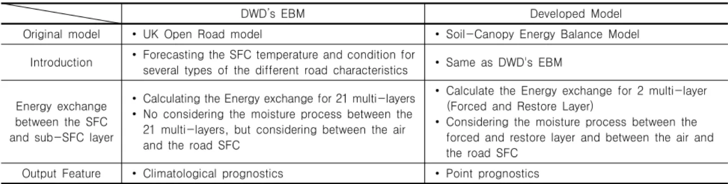
Table 1. Differences between the DWD’s EBM and the developed model
DWD’s EBM Developed Model
Original model ∙ UK Open Road model ∙ Soil-Canopy Energy Balance Model
Introduction ∙ Forecasting the SFC temperature and condition for
several types of the different road characteristics ∙ Same as DWD's EBM
Energy exchange between the SFC and sub-SFC layer
∙ Calculating the Energy exchange for 21 multi-layers
∙ No considering the moisture process between the 21 multi-layers, but considering between the air and the road SFC
∙ Calculate the Energy exchange for 2 multi-layer (Forced and Restore Layer)
∙ Considering the moisture process between the forced and restore layer and between the air and the road SFC
Output Feature ∙ Climatological prognostics ∙ Point prognostics
where is in unit cm (McCumver, 1980 ; Pielke, 1984) and the matric potential is,
(14)
where is the saturated moisture potential, and
the saturated volumetric moisture contents and b the slope of retention curve on logarithmic graph.
The volumetric heat capacity C is expressed by the density of the road soil, the specific heat and the soil moisture contents.
The ground heat flux can be calculated by the surface energy budget conservation theory. That is,
(15)
where is the sensible heat flux that is the function of friction velocity and friction temperature, the latent heat flux and the net radiation flux.
3. Verification of Model
To verify the developed model, its output was compared with the data from the German Weather Service (DWD), which utilizes the Energy Balance Model (EBM) based on the energy budget balance theory.
DWD’s EBM calculates the energy transfer through 21 sub-surface medium and classifies 160 types of the climatology for road condition. And 5 types of other road characteristics are considered.
We carry out the simulation for the L857 region (Hanau)
of Germany by using both DWD’s EBM and the developed model with the same initial conditions and period (November 2012~March 2013).
To compare the results of both models, the forecasted road surface temparatures of both models and the observed one are shown in Figs. 2 and 3.
The simulated results by using both models were very similar to each other and had a good match with the observed data. But the forecasted road surface temperature by using the developed model is about 1 K~2 K lower than that of DWD’s EBM. To find the cause of the under-estimation of the developed model, we checked the calculated several flux amounts. Major difference was that when the heat is transferred between the road surface and the subsurface layer, the response of the developed model (2-layer model) occurs more quickly than that of DWD’s EBM (multi-layer model). So, the minimum temperature is affected by the heat transfer rate.
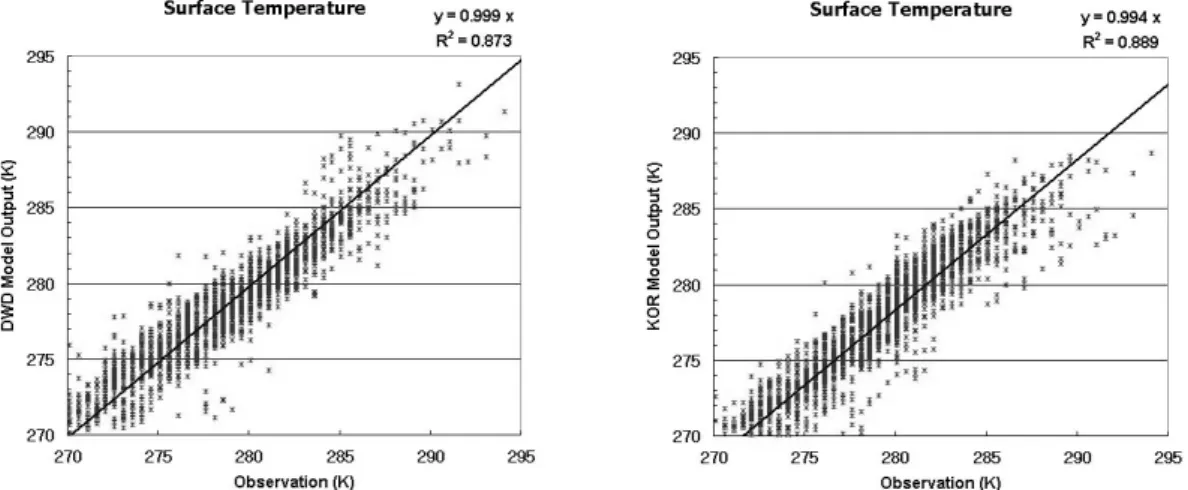
Two scatter diagrams and regression analysis results, which represent the relationship of the DWD’s EBM output, and those of the developed model and the observation, are shown at Fig. 3.
We can easily find that it is evident that the two model’s outputs and observed values are highly correlated, if the coefficient of determination R2 and the slope of regression line are nearly unitary. But the developed model’s output has a little bit cold bias as already discussed in previous chapter.
The developed model was run on 5 Oct., 2012, using the measurements of the KMA (Korea Meteorological Administration)’s pilot site which is located in Sindaebang-
Fig. 2. Time series of the calculated and observed road SFC temperature (DWD : calculated value by using the DWD’s EBM, KOR : calculated value by using the developed model, and Observation 1 and 2 : observed value on the observation site 1 and 2)
Fig. 3. Scatter diagram, regression line and regression analysis result for the modeled and observed road SFC temperature (DWD Model Output : calculated value by using the DWD’s EBM, KOR Model Output : calculated value by using the developed model, and Observation : observed value on the observation site)
dong, Seoul and the model outputs are compared with the observations data. The pilot site is composed of both the meteorological tower and road sensor which can measure the road SFC/sub-SFC temperature and road condition.
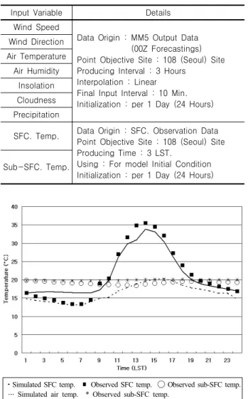
The simulated results (Fig. 4) utilizing the developed model were compatible with the observed data, within the error of less than 2 K. At the same time, the time lag between air temperature and road surface temperature
Table 2. Initial condition for the test run using the measurements of the pilot site
Input Variable Details
Wind Speed
Data Origin : MM5 Output Data (00Z Forecastings) Point Objective Site : 108 (Seoul) Site Producing Interval : 3 Hours
Interpolation : Linear Final Input Interval : 10 Min.
Initialization : per 1 Day (24 Hours) Wind Direction
Air Temperature Air Humidity
Insolation Cloudness Precipitation
SFC. Temp. Data Origin : SFC. Observation Data Point Objective Site : 108 (Seoul) Site Producing Time : 3 LST.
Using : For model Initial Condition Initialization : per 1 Day (24 Hours) Sub-SFC. Temp.
⁃ Simulated SFC temp. ∎ Observed SFC temp. ◯ Observed sub-SFC temp.
… Simulated air temp. * Observed sub-SFC temp.
Fig. 4. Calculated road surface temperature and subsurface temperature by using the developed model and Observed data
(about 3∼4 LST) was also well simulated by the model, as the measurement shows.
The numerical weather forecasting output from KMA/
MM5 was used as the synoptic input data, for running model. Because of the initial error of the MM5 output, the simulated road surface temperature and ground temperature showed the difference in values from the measurement.
As a result, the quality of road surface condition was found to be dependent on the quality of the NWP, when we operated the Energy Balance Model for road weather prediction.
4. Conclusion
The prognostic model for the prediction of the road
surface temperature is developed using the surface energy balance theory. And the developed model output is compared with DWD’s EBM outputs and the pilot site’s observations to verify the developed model’s performance.
The simulated results by using both model were very similar to each other and were compatible with the observed one. But the developed model underestimates the minimum road surface temperature rather than DWD’s EBM.
If the developed model is improved to have more subsurface layer, more accurate result will be produced.
References
1. Atkinson, B. W. (1981), Meso-Scale Atmospheric Circulations.
Atmospheric Press, London.
2. Betchtold, P., J. P. Pinty and P. Mascart (1991), A numerical investigation of the influence of large-scale winds on sea-breeze/
land-breeze type circulation. J. appl. Met., 30, pp.1268-1279.
3. Bhumralkar, C. M. (1975), Numerical experiments on the computation of the ground surface temperature in atmospheric general circulation model. J. Appl. Meteor., 14, pp.67-100.
4. Blackadar, A. K. (1976), Modeling nocturnal boundary layer. Proc.
3rd Symposium on Atmos. Turbulence, diffusion, and air quality, Raleigh, NC, Amer. Meteor. Soc., pp.46-49.
5. Brutsaert, W. (1982), Evaporation into the atmosphere: Thoery, History and Application D. Reidel Publishing Company, Dordrecht.
6. Carson, D. J. (1982), Current parameterization of land-surface processes in atmospheric general circulation models, Ed. by Eagleson, C.U.P., London, pp.67-108.
7. Du, J., Song, K., Wang, Z., Zhang, B. and Liu, D. (2013), Evapotranspiration estimation based od MODIS products and surface energy balance algorithms for land(SEBAL) model in Sanjiang Plain, Northeast China, Chinese Geographical Science, 23:1, pp.73-91.
8. Garratt, J. P. (1992), The atmospheric boundary layer. Cambridge Univ. Press. 316pp.
9. Gutierrez, M.V. and Meinzer, F.C. (1994), Energy balance and latent heat flux partitioning in coffee hedgerows at different stages of canopy development, Agric. Forestry Meteorol., 68, pp.173-186.
10. Lagos, L.O., Martin, D.L., Verma, S.B., Suyker, A. and Irmak, S. (2011), Surface energy balance model of transpiration from variable canopy cover and evaporation from reside-covered or bare-soil systems: model evaluation, Irrigation Science, 31:2, pp.
135-150.
11. McCumber, M.C. (1980), A numerical simulation of the influence of heat and moisure fluxes upon mesoscale circulations. Ph.D.
dissertation, Dept. of Environmental Science, Univ of Virginia, Charlottesville, 255pp.
12. Monteith, J.L. (1981), Evaporation and surface temperature. Quart.
J. Roy. Meteor. Soc., 107, pp.1-27.
13. Noihan, J. M. and S. Planton (1989), A simple parameterization of land surface processes for meteorological models. Mon. Wea.
Rev., 117, pp.536-549.
14. Park, S.-U. (1994). The effect of surface physical conditions on the growth of the atmospheric boundary layer. J. Kor. Meteor.
Soc., 30(1), pp.119-134.
15. Pielke, R. A. (1984), Mesoscale meteorological modeling. Academic Press, New York, pp.612.
16. Sato (2009), Road surface temperature forecasting (case study in mountainous region of Japan), Proceeding of cold region technology conference, pp.382-388.
17. Schmugge, T. and Humes, K. (1995), Aster observations for the monitoring of land surface fluxes, J. Jap. Remote Sensing Soc., 15, pp.83-89.
18. Segal, M., W. E. Schreiber, G. Kallos, J. R. Garratt, A. Rodi, J.
Weaver and R. A. Pielke, (1989), The impact of crop areas in
northeast Colorado on midsummer mesoscale thermal circulations.
Mon. Wea. Rev., 117, pp.809-825.
19. Senay, G.B., Budde, M.E. and Verdin, J.P. (2010), Enhancing the simplified surface energy balance (SSEB) approach for estimating landscape ET: Validation with the METRIC model, Agricultural Water Management, 98:4, pp.606-618.
20. Zhihao, Q., Pedro, B. and Arnon, K. (2002), Numerical solution of a complete surface energy balance model for simulation of heat fluxes and surface temperature under bare soil environment, Applied Mathematics and Computation, 130:1, pp.171-200.
Received : March 28th, 2014 Revised : August 4th, 2014 Accepted : November 3rd, 2014