1. Introduction
In july 27, 2011, a catastrophic debris flow happened on Mt. Majeok in the Cheonjeon-ri area in Chuncheon city in Gangwon province, which led to deaths of 10 college students and three adults, and 26 injuries. The catastrophe was caused by torrential rain, itself caused by recent extreme weather.
Antecedent rainfall prior to the landslide was approximately 525mm, and rainfall on the day of the incident was 255mm; the recorded rainfall surpassed the landslide alert level. South Korea has a high risk of accidents from landslides, because most land is mountainous, the population density is very high, and housing, roads, and social infrastructure are often close to mountains (Kim, 2013). In addition, most accidents occur in summer when torrential rain frequently occurs, because the country is located in a meteorologically heavy rain area. Since most domestic landslides are caused by torrential rain in
the summer, evaluation with a technique that estimates the extent of damage that takes the inherent characteristics into account and reliable simulation techniques both need to be conducted. Oh et al.(2009) analyzed topographical and hydrological effect of debris flow movement which is affected by initiation, flow and deposition using Satellite image.
Wie et al.(2010) extracted slope, flow direction and contour from DEM to simulate movement of sediment according to lapse of time using finite different method. Scheuner et al.(2011) simulated the runout distance, velocity, flow depth and impact pressure of debris flows from Mattenbach, Stechelberg in Switzerland using RAMMS two- dimensional debris flow model. LIN et al.(2011) estimated debris flow hazard area using FLO-2D model.
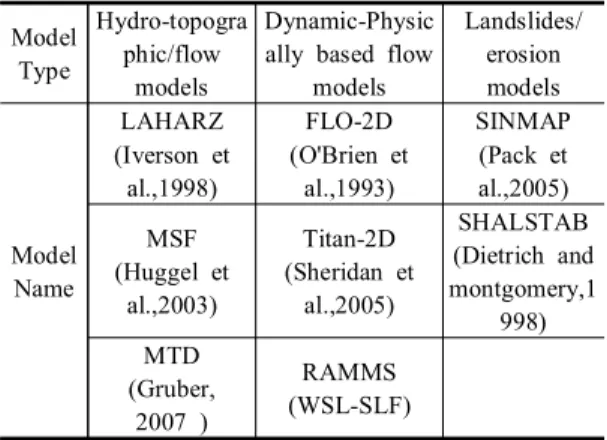
Table 1 shows classification of mass movement simulation model. This study aims to evaluate the feasibility of a GIS technique that considers the soil
Received: 2016.04.14, revised: 2016.06.13, accepted: 2016.06.15
* MemberㆍPh.D Candidate, Department of Civil Engineering, Sungkyunkwan University, [email protected]
** Corresponding AuthorㆍMemberㆍProfessor, Department of Civil Engineering, Sungkyunkwan University, [email protected]
*** Ph.D Candidate, Department of Aero Mechnical Engineering, Sungkyunkwan University, [email protected]
A Study on the Debris Flow Hazard Mapping Method using SINMAP and FLO-2D
1)
Kim, Tae Yun*ㆍYun, Hong Sic**ㆍKwon, Jung Hwan***
Abstract
This study conducted an evaluation of the extent of debris flow damage using SINMAP, which is slope stability analysis software based on the infinite slope stability method, and FLO-2D, a hydraulic debris flow analysis program. Mt. Majeok located in Chuncheon city in the Gangwon province was selected as the study area to compare the study results with an actual 2011 case. The stability of the slope was evaluated using a DEM of 1 x 1m resolution based on the LiDAR survey method, and the initiation points of the debris flow were estimated by analyzing the overlaps with the drainage network, based on watershed analysis. In addition, the study used measured data from the actual case in the simulation instead of existing empirical equations to obtain simulation results with high reliability. The simulation results for the impact of the debris flow showed a 2.2-29.6% difference from the measured data. The results suggest that the extent of damage can be effectively estimated if the parameter setting for the models and the debris flow initiation point estimation are based on measured data. It is expected that the evaluation method of this study can be used in the future as a useful hazard mapping technique among GIS-based risk mapping techniques.
Keywords : Landslide, Debris Flow, SINMAP, FLO-2D, Hazard Mapping
15 Vol.24 No.2 June 2016 pp.15-24
Research Paper
ISSN: 2287-6693(Online) http://dx.doi.org/10.7319/kogsis.2016.24.2.015
Model Type
Hydro-topogra phic/flow
models
Dynamic-Physic ally based flow
models
Landslides/
erosion models
Model Name
LAHARZ (Iverson et
al.,1998)
FLO-2D (O'Brien et
al.,1993)
SINMAP (Pack et al.,2005) MSF
(Huggel et al.,2003)
Titan-2D (Sheridan et
al.,2005)
SHALSTAB (Dietrich and montgomery,1
998) MTD
(Gruber, 2007 )
RAMMS (WSL-SLF)
Table 1. Classification of Mass Movement Simulation Model
characteristics of a study area and the rainfall at the time of an accident by estimating the extent of damage of a debris flow and comparing it with an actual case to provide a technique as a future direction for the application of GIS-based hazard mapping.
1.1 Selection of Study Area and Research Methods
This study selects Mt. Majeok as the study area, it is located in Cheonjeon-ri in Chuncheon city in the Gangwon province, and was the site of a debris flow that generated an enormous amount of damage in 2011. The stability of the slope was evaluated using a DEM with 1 x 1 m resolution based on aerial LiDAR survey approach to analyze the debris flow of the study area, and debris flow initiation points were
Figure 1. Flow-Chart of Study
estimated using overlapping analysis with the results of watershed analysis. In addition, a hydraulic simulation of a debris flow was conducted using numerical analysis software based on a rheological model that takes into account the rainfall at the time of accident. A comparative analysis of the simulation results and the actual data from the time of the accident was performed to evaluate the technique’s feasibility. Fig. 1 is a flowchart that outlines this study.
2. Causes of Landslides
Prior to the analysis of the debris flow, the causes of landslides, considered a higher-order concept of debris flow, should be examined. Landslides occur due to complex mechanisms of various internal and external factors. Internal factors refer to static factors of environment with little influence such as the terrain, geology, and soil, whereas external environmental factors refer to factors that cause landslides through external impacts such as rainfall and earthquakes (Yang et al., 2007).
This study conducts simulations on the extent of damage of a debris flow by taking into account both the internal factors of terrain, geology, and soil, and the external factor of rainfall.
3. Analysis of Characteristics of Debris Flow Development in Study Area
3.1 Classification of Debris Flow by Type of Development
The most common form of sediment movement
caused by landslides in Korea is debris flow. Debris
flow can be classified into either hill slope debris
flow or channelized debris flow depending on the
form of its development (Winter et al. 2005). In a
study on the behavior characteristics and sizes of
debris flows, Zhang (2010) classified debris flows
observed in the Gangwon province, which includes
the study area of the present study, into the types
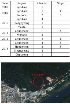
described in Table 2. It was determined that the
proportion of channelized debris flows in the
Gangwon province was 71.1%.
Year Region Channel Slope
2008 Inje-Gun 5
2009 Inje-Gun 5 1
Jechoen 2 2
2010
Inje-Gun 4
Yangpyeong 1
YeoJu 1
2011 Chuncheon 5
Milyang 2
2012 Chuncheon 3 1
2013
Chuncheon 4 3
Hongcheon 2 3
Hoengseong 2
Gapyeong 1
Table 2. Classification of Debris Flow Initiation shape in Kangwondo
Figure 2. Observed Initiation Point
The inclination of the slope is also an important factor in the development of debris flow. According to Kim and Chae (2009), landslides occur most commonly at 26–30° and 31–35°; Mt. Majeok (Fig.
2) had two landslides at 15 minute intervals start at a site approximately 150 m in height at inclination 30–35°, which is consistent with the ranges of typical inclinations for landslide development surveyed in the study.
3.2 Initiation Mechanism of Debris Flow Takahashi (2007) classified the causes of debris flows initiated in the event of torrential rain in mountainous areas with steep hills into the following categories: (1) destruction of a natural slope, (2) scouring and erosion at the bottom and the sides of a valley, and (3) the collapse of a natural dam of sediment. The destruction of a natural slope in Korea
Figure 3. Concept of Debris Flow Initiation
is initiated by increased pore pressure due to the infiltration of rainfall, which is similar to the circumstances encountered in Japan. Taking this into account, this study makes the following assumptions to estimate the initiation points of the debris flow:
(1) When it rains, rainwater is primarily collected through a drainage network that temporarily forms with many streams on the slope, into the catchment area, forming a channel and moving on to the slope, and (2) debris flow is likely to develop in areas that are rated low on the Stability Index, the result of the stability assessment of the slope. Fig. 3 shows the concepts used in the estimation process of debris flow initiation points proposed by this study.
3.3 Debris Flowing Mechanism
Made up of fine particles, sediments maintain slopes in a state of cohesion, and the flow of fluid generated from rainfall creates shear stress in four directions. When the shear stress becomes larger than the yield stress limit created by cohesive pressure, sediment particles and water mix move. The flow of debris can be considered as a movement of fluid with cohesive pressure, and rheological features such as yield stress and cohesion can be an important determinant of the fluidity of a destroyed slope (Jeong, 2010).
This study simulated the movement of the extent of
damage of debris flow as a function of specific
sediment concentrations using FLO-2D model to
incorporate the behavioral characteristics of a debris
flow. The governing equations of the FLO-2D model
are the continuity equation designated as Eq. (1) and
the momentum equation explicated by Eqs. (2) and
(3).
(1)
= Depth of debris flow (m),
= Average flow rate in
the direction of the axis (m/s),
= Average flow rate in
the direction of the axis (m/s),
= Rainfall intensity (mm/hr)
(2)
(3)
,
: Respective friction slopes in the axis and axis directions.
,
: Respective bed slopes in the axis and axis directions.
: Acceleration due to gravity (9.81 m/s2)
3.4 LiDAR DEM
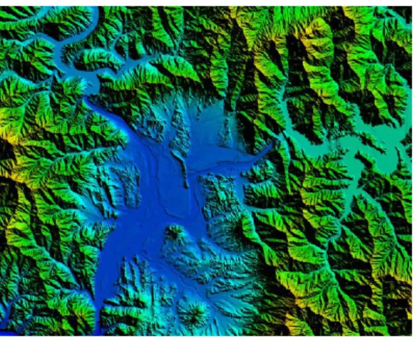
A DEM of 1 x 1 m resolution obtained from aerial LiDAR survey method was used to obtain the topographic data used in this study. The aerial LiDAR system generates terrain data on the Earth’s surface by shooting laser pulses from an aircraft equipped with a laser scanner, measuring the time required for the pulses to reach the surface, and calculating the three-dimensional coordinates of the spots at which the pulses are reflected. Recently, it has demonstrated an accuracy of 0.089 m ± 0.062 m
Figure 4. Chuncheon 1m × 1m resolution DEM
on average for orthometric heights on conventional digital maps, using a GPS/INS based unified approach, and was found to be superior to 1/1,000 digital maps (Wie et al. 2007).
This method can also produce DEM, DSM, contour lines, and shaded relief maps by extracting the coordinates of point-clouds obtained from aerial LiDAR survey from preprocessing with GPS/INS, and post-processing irregular point data. Fig. 4 shows the DEM of Chuncheon city, which was used in this study.
4. Slope Stability Analysis
4.1 SINMAP Parameter Setting
This study used SINMAP as a model for evaluating slope stability. Table 3 shows the parameters that were set up based on the results of Seo (2012), which conducted an indoor experiment with soil sampled from two randomly selected spots in the area at which the accident occurred during the landslide, instead of the initial parameter values commonly used in such analysis.
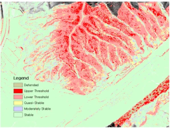
The analysis results are expressed as the Stability Index, which indicates the stability of the slope at each spot in relation to the development of debris flow. The Stability Index indicates relative risk instead of an absolute value for the precise risk, and the red zone shown in Fig. 5 (i.e., the zone of Upper Threshold 0.0 < SI < 0.5) is assumed a low stability zone and designated as a zone with a high probability of flow debris.
Variables Value Unit
Gravity Constant 9.81 m/s
2Water Density 1000 kg/m
3Ratio of
Transmissivity 60~200 m
Soil Cohesion 0.1~0.23 t/m
2Soil Friction Angle 38~40 °
Soil Density 1763 kg/m
3Table 3. Parameters of SINMAP Analysis
Figure 5. Stability Index of Mt. Majeok
4.2 Watershed Analysis
Based on the concept map of Fig. 3, this study developed a virtual drainage network in all four directions by performing watershed analysis at 1 x 1 m resolution to estimate the catchment area that temporarily forms during a rainfall event. The spot with highest probability of developing debris flow was estimated for each watershed by marking the formed network in blue and performing overlap analysis on the network with the zone of Upper Threshold 0.0 < SI < 0.5 in red, and the area of threshold saturation in green. Fig. 6 shows the debris flow initiation point for each watershed, as estimated from overlap analysis.
Figure 6. Debris Flow Initiation Point
5. Debris Flow Movement Simulation
5.1 FLO-2D Model Parameter Setting 5.1.1 Sediment Concentration
One of the most important factors in debris flow simulation is sediment concentration. The state of the fluid is determined by the sediment concentration in FLO-2D simulation, and debris flow takes a value of 0.45–0.55 volume concentration according to the classification in Fig. 7. When the concentration is lower, sediment moves faster and spreads wider. A concentration of 0.52 was used in this study, considering that the debris flow took the form of hill slope flow debris, which has relatively larger sediment particles.
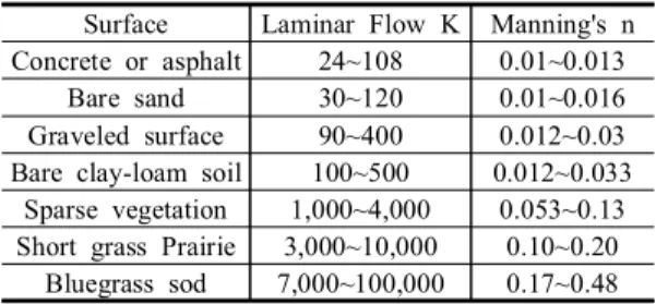
5.1.2 Manning's n Value and Laminar Flow K Since the debris flow that flows down the slope shows the hydraulic behavior of a fluid with viscosity, the hydraulic roughness of the slope as a path must be considered. Manning's n is the value set for each calculation grid to indicate the coating state of the ground surface, and is set at 0.07 based on the data from Woolhiser (1975) in Table 4 and data from a previous study that conducted a geological survey of the site. In addition, the laminar flow resistance parameter K was set at 3500 in consideration of the forestry distribution of the study area.
Figure 7. Classification of Flow Status
Surface Laminar Flow K Manning's n Concrete or asphalt 24~108 0.01~0.013
Bare sand 30~120 0.01~0.016
Graveled surface 90~400 0.012~0.03 Bare clay-loam soil 100~500 0.012~0.033
Sparse vegetation 1,000~4,000 0.053~0.13 Short grass Prairie 3,000~10,000 0.10~0.20
Bluegrass sod 7,000~100,000 0.17~0.48 Table 4. Manning's n Value & K Parameters
5.1.3 Yield Stress and Coefficient of Viscosity The FLO-2D model provides empirical coefficients on yield stress, viscosity, and sediment concentration.
O'Brien and Julien (1988) expressed the relationships between the volume concentration Cv and the coefficients obtained from rheological analysis—yield stress and viscosity—as Eqs. (4) and (5).
(4)
(5)
Hubl and Steinwendtner (2001) concluded that the most important factors in FLO-2D simulation are the digital terrain and rheological parameters (i.e., yield stress and the coefficient of viscosity). When it was impossible to obtain samples from actual sites, previous studies estimated the yield stress and the coefficient of viscosity using O'Brien’s empirical coefficients provided by the FLO-2D model;
however, the present study’s parameters are the estimates for yield stress and volume concentration based on the soil properties of the study area measured using linear regression analysis in “Yield Stress and Viscosity Characteristics of Soils with Liquidity Index” (Kang et al., 2013) to increase the
credibility of the parameter selection. In Table 5, Soil Sample Cases 1 and 2 are measurements of the samples obtained from two randomly selected spots in the area of the accident, which were used in SINMAP analysis, and Case 3 is O'Brien’s empirical coefficients for Glenwood, which have been used in many previous studies, and are used in the present study for comparison purposes.
Soil Sample
(Pa)
(Pa·s)