1. Introduction
Sediment is one of the most difficult water quality constituents to accurately represent in current watershed and river model. Important aspects of sediment behavior within
a watershed system include loading and erosion source, delivery of these eroded sediment sources to river, drains and deposition processes. Sediment finally reach to coastal zone by of river path. In connection with the coastal erosion, Phillips has pointed out that rivers are the major source of coastal sediment (Phillips, 1995). The sediment in coastal areas represents evidence of changes from river sediment delivery driven by human or natural impacts. Urbanization
Estimating magnitude of suspended sediment transport in ungauged east coastal zone
Lee, SangeunaㆍKang, Sanghyeokb*
aDepartment of Energy and Mineral Resources Engineering, Kangwon National University
bDepartment of Earth Environmental System Engineering, Kangwon National University
Paper number: 17-083
Received: 14 October 2017; Revised: 3 December 2017; Accepted: 3 December 2017
Abstract
Coastal sediment archives are used as indicators of changes on shore sediment production and fluvial sediment transport, but rivers crossing coastal plains may not be efficient conveyors of sediment to the coast. In some case there is a net loss of sediment in lower coastal plain reaches, so that sediment input from an upstream exceeds the sediment yield (SY) at the river mouth. The main source of sediment in coastal area is the load from land. In Korea, data on suspended SY are limited owing to a lack of logistic support for systematic sediment sampling activities. This paper presents an integrated approach to estimate SY for ungauged coastal basins, using a soil erosion model and a sediment delivery ratio (SDR) model. For applying the SDR model, a basin specific parameter was validated on the basis of field data. The proposed relationships may be considered useful for predicting suspended SY in ungauged basins that have geologic, climatic and hydrologic conditions similar to the study area.
Keywords: Ungauged coastal basin, Sediment delivery ratio, Coastal area
미계측 동해안 유역의 토사유출 규모의 평가에 관한 연구
이상은aㆍ강상혁b*
a강원대학교 에너지 자원공학과, b강원대학교 지구환경공학과
요 지
토사유출에 대한 자료는 극히 제한되어 있으며 이에 대한 관측지점 또한 대하천에 국한되어 있다. 더욱이 대하천 하류의 해안부근 유사량 자료는
전무한 실정이다. 본 연구는 지속적인 토사유입으로 인하여 그 면적이 줄어들고 있는 동해안의 석호인 유역면적 8.2km2의 향호를 대상으로 토사량
유출량을 계산하여 유호성을 검증하였다. 그 결과 향호로 유입되는 비유사량은 약 280 t/km2/yr 이었으며 유사전달률은 약 0.78이었다. 본 접근 방법은 현재 육역화가 대부분 진행되어 있는 동해안 석호의 토사유입 과정을 유추하는데 유효한 자료가 될 것으로 기대한다.
핵심용어: 미계측유역, 유사전달률, 연안지역
© 2018 Korea Water Resources Association. All rights reserved.
*Corresponding Author. Tel: +82-33-570-6570 E-mail: [email protected] (S. Kang)
affects this equilibrium by decreasing, slowing, and halting the movement of sediment to coastal areas. This is an important issue for many coastal regions around the world (Fernandez et al., 2003; Ferro and Porto, 2000). It is also becoming increasingly obvious that sediment loads in the world’s rivers have been impacted by human development.
Although some specific zones have abundant SY data, in practice sediment yield data are very limited in the coastal area due to lack of high cost sediment data collection. This paper synthesizes calculated SY in ungauged basin and newly-derived power function Eq. based on measured SY data. And then this study was conducted to determine the runoff of SY in selected sub-river basin of the Meaho.
2. Study area and data collection
South Korea (S. Korea) is surrounded by sea on three sides, with 11,542 km of coastline. Most beaches on the east coast are clayey tidal flats. The tide is semidiurnal with maximum range of about 10 m. On the other hand, most beaches on the east coast are sandy beaches that have been suffering from beach erosion. The coastal region is the most dynamic part of the seascape since its shape is affected by various factors, such as hydrography, geology, climate, and vegetation.
Coastal erosion may be caused by natural processes such as waves, currents, and storms as well as human activities such as land reclamation, recreation at beaches, and construction of infrastructure in coastal areas (Rosati, 2005).
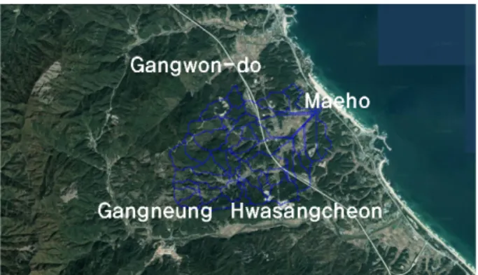
The study area is located on the East coastal side of S.
Korea, having 8.2km2 of basin as shown in Fig. 1. The Maeho
formed from lagoon lies to the end of basin. The present investigations were conducted on the East Sea of S. Korea between both headlands. The coast has a flat slope (1/200) with a narrow beach that ranges from 5 m to 75 m wide. The annual mean rainfall is 1,200 mm, which varies by typhoon.
Since 1998, rapid urbanization due to increased population caused intensive construction of buildings, roads and other infrastructures very close to the coastal area. The impacts of urbanization on the coastal area were reviewed by various researchers (Fu et al., 2006; Jain and Kothyari, 2000). Attacks from typhoons sometimes caused a great deal of damage to the region.
In order to analyze the characteristics of soil erosion within the basin and the cause of SY, a soil erosion model requires information on the digital elevation model (DEM), soil, and land cover. To determine the geomorphological character- istics, we developed a triangle irregular network (TIN) using a 1:5,000 scale digital topographic map crafted by the National Geographic Information Institute (NGII). Using the TIN, a 10 m resolution DEM was developed because it is closest to the typical Revised Universal Soil Loss Equation (RUSLE) resolution of 22 m. The land cover of the 1980 and 2005 data was processed using 30 m resolution LANDSAT satellite images by Water Management Information System (WAMIS).
3. Methodology
3.1 Soil erosion
RUSLE is used as a soil erosion model to estimate the amount of soil erosion from basins (Kothyari and Jain, 1997).
As the theoretical basis of RUSLE has been clearly reported elsewhere (Lee and Kang, 2014), we provide here only a brief description of the model. In the RUSLE, the amount of soil loss is a product of five factors representing the rainfall and basin characteristics, as follows;
⋅⋅⋅⋅ (1)
where, is the gross amount of soil erosion in cell (t ha-1 year-1); R is the rainfall erosivity factor (MJ mm ha-1 h-1 year-1);
Fig. 1. Location map showing Maeho basins
K is the soil erodibility factor (Tons ha h ha-1 MJ-1 mm-1); LS represent slope length and slope steepness (dimensionless);
C is the cover management factor (dimensionless); and P is the supporting practice factor (dimensionless).
R is generally calculated from an annual summation of rainfall data using rainfall energy over 30-min duration. On annual basis, the EI30 value as an erosivity factor is the sum of values over the storms in an individual year. The erosivity of rainfall varies greatly by location because of the effects of elevation in rainfall. Wischmeier and Smith (1978) observed that there's a high correlation between rainfall kinetic energy and its maximum intensity, EI30 and the amount of soil eroded. Erosivity factor is an indication of the two most important characteristics of a storm determining its erosivity:
amount of rainfall and peak intensity sustained over an extended period.
Some researchers evaluated the erosivity and developed statistical relationship between R-factor and the total annual precipitation (Pal et al., 2012). As there are limited meteoro- logical stations in mountainous basin, information on rainfall amount and pattern needs to be assumed based on neighboring stations (Lee and Kang, 2013). The rainfall information available represents point data, and this has to be extrapolated in terms of spatial distribution, using the Arc GIS contouring function. In this study, the Eq. (2), developed by Korea Institute of Construction Technology KICT (1992), was used for computing the R factor as:
(2)
where, Pr is the average annual precipitation of the study area.
The erodibility of a soil K is an expression of its inherent resistance to detachment and transport by rainfall (Wischmeier et al., 1971). It is determined by the cohesive force between the soil particles. Soil erodibility may vary depending on soil characteristics, such as particle distribution, soil structure, and organic matter, etc. The formula for soil erodibility (Kamaludin et al., 2013) is as follows:
× ×
(3)
where, OM is organic matter (%), N1 is clay+very fine sand (0.002-0.125 mm), N2 is clay+very fine sand+sand (0.125-2 mm), SS is soil structure code, and PP is profile permeability class (Wischmeier and Smith, 1978).
Korean National Academy of Agricultural Science published the soil map with 1:50,000 scales (KNAAS, 2014).
Based on this map, a digital soil map was produced with the ArcGIS coverage of the 1:25,000 scales. Soil classification in study area was divided into 59 types of total 390 soil types.
LS are the slope length and gradient factor. The slope length and slope steepness can be used in a single index, which expresses the ratio of soil loss as defined by Wischmeier and Smith (1978) as:
(4)
where, X is the slope length (m), m is slope length exponent, and S is slope gradient (%). In order to calculate X value, Flow Accumulation was derived from DEM after conducting Fill and Flow Direction processes in ArcGIS. The vegetation cover factor C represents the ratio of soil loss under a given vegetation cover as opposed to that on bare soil. The vegetation cover intercepts raindrops and dissipates its kinetic energy before it reaches the ground surface (Renard et al., 1997). The relative impact of management options can easily be compared by making changes in the C factor which varies from near zero for well protected land cover to one for the barren areas (Lee and Lee, 2006). The effect of contouring and tillage practices on soil erosion is described by the support practice factor P within the RUSLE model (Renard et al., 1997). Wischmeier and Smith (1998) defined the support practice factor P as the ratio of soil loss with a specific support practice to the corresponding soil loss due to up and down cultivation. If there are no support practices, the P factor is 1.00. Contemporary agricultural practices consist of up and down tillage without the presence of contours, strip cropping, or terracing. The P factor depends on the conservation measure applied to the study area. In this study, the factors C and P were applied on the basis of KICT (1992) classification.
3.2 River sediment yield model
SY is the amount of solid particles that is delivered to the
outlet of the basin. SY at a mouth of the basin is calculated by multiplying gross erosion above that point by a SDR. The SY load from each measurement can be derived as:
⋅ (5)
where, is suspended sediment load (t/day), is water discharge (m3/s), is sediment concentration (mg/l)
Calculating the annual sediment load of a river can be quite straightforward, if discharge and sediment concentration are measured at closely spaced intervals, particularly during floods. In most cases, however, a continuous record of sediment concentration is not available, and indirect methods must be utilized using a sediment rating curve (SRC). The SRC is a widely adopted method for estimating sediment concentration and load (Yekta et al., 2010). As sediment concentration and load often vary over several orders of magnitude, the SRC is generally established by a power function (Lu and Siew, 2005) that relates available sediment load () to water discharge ():
(6)
where, a is regression constant and b is slope by regression analysis.
3.3 Review of sediment delivery ratio
The SDR is the ratio of SY at the outlet, over the total volume of produced sediment using Eq. (5) in the drainage basin. It is well known that the SDR is related to basin size, i.e. it decreases with the size of basin. There are some methods to estimate SDR, namely an observed SRC model linking RUSLE, and a combination of the SEdiment Delivery Distribution (SEDD) model and RUSLE model (Lee and Kang, 2014). The SDR values can be assessed with GIS- based spatially distributed sediment models using field experimental data.
3.3.1 SDR model coupling RUSLE and SRC
RUSLE is a basin model; thus it cannot be directly used to estimate the amount of sediment reaching downstream areas, because some portion of the eroded soil may be
deposited while traveling to the watershed outlet or the downstream point of interest (Neibling and Foster, 1977). To account for these processes, the SDR for a given watershed should be used to estimate the total sediment transported to the watershed outlet. The SDR can be expressed as follows:
(7)
3.3.2 SEDD model
Empirical Equations for SDR are usually based on variables, such as basin area, slope and land cover (Ferro and porto, 2000). For example, Kothyari and Jain (1997) estimated the SDR values from the watershed area, relief ratio and average runoff curve number value. They applied a lumped approach, but improved this by division of the modeled basin into smaller watersheds. According to some authors (Mutua and Klik, 2006), the coefficient, which is a measure of the probability that the eroded particles are transferred from the morphological unit under consideration to the nearest stream reach, can be generalized as follows:
exp exp
exp
(8)where, is basin specific parameter depends on morpho- logical data, is travel time (hr) of overland flow from the
overland cell to the nearest channel cell down the drainage path.
If the flow path from cell i to the nearest channel traverses Np cells, then the travel time from that cell is calculated by adding the travel time for each of the Np cells located along the flow path. is the length of segment i in the flow path (m), and is equal to the length of the side or diagonal of a cell, depending on the flow direction in the cell. is the flow velocity for the cell (m/s). The flow velocity is considered to be a function of the land surface slope and the land cover characteristics, i. e. × . If is the amount of soil erosion produced within the cell of the basin estimated using Eq. (1), then the SY for the basin, SY, is obtained, as below:
⋅ (9)
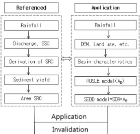
where, n is the total number of cells over the basin. Since the SDR of a cell is hypothesized as a function of travel time to the nearest channel, this implies that the gross erosion in that cell multiplied by the SDR value of the cell becomes the SY contribution of that cell to the nearest stream channel. The SDR values for the cells marked as channel cells are assumed to be unity. SY modeling is a more complicated and time- consuming process, since the RUSLE method cannot drive the SY directly. In order to estimate the SY, then we combine the RUSLE and SDR model, using the Model Builder (MB) in the ArcGIS environment. Simulated SY was validated with observed one as shown in Fig. 2.
4. Results
4.1 Soil erosion
In order to calculate SDR by modeling, the relationship between soil loss and SY needs to be determined. The annual soil erosion from each identified grid of the basin was computed by integration of the RUSLE erosion factors, namely R, K, LS, C and P of RUSLE. The values of the RUSLE parameters were integrated in ArcGIS, using a Raster Calculator to form a composite map denoting gross soil erosion, based on 30 m DEM. Land use data of 30 × 30 m, provided by the Water Management Information System in 1980and 2015, was reclassified to create a new map with the following categories: (a) water, (b) urban, (c) barren, (d) wetland, (e) pasture, (f) forest, (g) paddy farming, and (h) field crop area. The soil classification map of the study area was divided into 59 soil types such as Afa, Ana, Apa, Rea, Maa, Ro, etc. In 1973, the NAAS published the soil map at a scale of 1:50,000. Based on this paper map, a digital soil map was produced with the ArcGIS coverage of a 1:25,000 scale. Rainfall erosivity is determined by climatic data. For calculating R factors in the study basins, we used an annual average value using the isohyetal method (Lee and Kang, 2013) based on 59 meteorological observation stations.
Changes occurring in the values of the factor C due to crop growth over such a small duration were neglected (Mutua and Klik, 2006). In this study, the factors C and P were applied on the basis of KICT (1992) classification.
Computed values of average annual erosions of Maeho basin are presented in Fig. 3. The annual average soil erosion for the Maeho basin ranged from 320 to 333 tons/km2/yr for
Fig. 2. Model validation process between calculated and observed sediment yields using model builder of ArcGIS
Fig. 3. Soil erosion potential map of Maeho basin
the two years of 1980 and 2015. These values are slightly lower than those obtained by Lee and Kang (2014), probably as a consequence of using a DEM to calculate length-slope factors.
4.2 Sediment load to ungauged coastal basin and validation
In order to estimate the variation of SY in the ungauged coastal regions, SDR was derived from Eq. (8). SY is the function of SDR and Soil erosion. It is well known that an inverse relationship exists between SDR and the basin area.
SDR generally increases with decreasing basin size. The SDR in the field approaches 100% for small and urbanized basins (Lee and Kang, 2014) as shown in Fig. 4.
According to preceding research the steepest areas of a basin are the main sediment producing zones, and since
average slope decreases with increasing basin size the sediment production per unit grid decreasing too. Large basins also have more sediment storage sites located between sediment source area and the basin outlet (Kang, 2015).
After the values of RUSLE and SDR were derived, SY was calculated using Eq. (9). As shown in Fig. 5, SY was calculated to range from 2,300 to 2,400 t/ha for the ungauged Maeho basin, during two years of 1980 and 2015. And the computed SY in the study basin for the two years are summarized as shown in Table 1.
Otherwise, in other to estimate annual SY, a SRC was derived as a linear regression using Eq. (5), on the basis of reference data. As sediment concentration and load often vary over several orders of magnitude, the SRC is generally established by a power function (Lee and Kang, 2014) that relates available sediment load (QS) to water discharge (QW):
(10)
where, is regression constant and is slope by regression analysis.
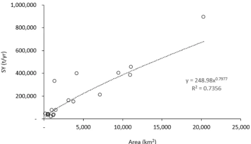
Fig. 6 shows discharge of SY with basin area using published data. If the basin size of the Maeho is 8.2 km2, the SY may be 1,333 (t/yr) by power function of Eq. (10), approximately. The SY calculated from the Eq. (10) has a lower value than the modeled owns. We can estimate that it
Fig. 4. Comparison of different relations between SDR and basins
Fig. 5. Sediment yield map of Maeho basin Table 1. Annual sediment transport for ungauged coastal basin
Basin Area Soil loss (t/yr) SDR Sediment yield (t/yr)
1980 2015 1980 2015 1980 2015
Maeho basin 8.2 2,600 2,700 0.79 0.81 2,300 2,400
is because of a long period (December to next March) of the whole year has a melting season, with little or no rainfall in S.Korea. Over 80% of total SY is concentrated on wet monsoon periods and it will reduce the SY to rivers.
The Specific Sediment Yield (SSY) of 17 rivers in Korean basins ranged from 34 to 213 t km-2yr-1 (Lee and Kang, 2014).
These SSY values are similar trend to that of a previous result obtained by Milliman and Syvitski (1992) for 22 Asian river basins from 25 to 250 t km-2yr-1 as shown in Fig. 7.
5. Conclusions
The SY, especially in coastal areas, is too sensitive to readily obtain data. Their data has been scarcely used, because its conventional measurement methods are expensive and time-consuming. In this paper, a theoretically
based relationship for evaluating the soil loss and SDR is proposed to estimate SY in an ungauged basin. Soil erosion in the individual cells of the basin was determined using the RUSLE. The value of SDR was calibrated comparing the calculated SY for the study basins and similar observed basins, as defined by Eq. (8). The annual SDR at the outlet of the basin was estimated in the range from 0.75 to 0.81 for the Maeho basin. The calculated SSY ranged from 271 to 296 t/km2/yr for the Maeho. The method depends on calibration against a record of existing conditions and hence it can be used for the estimation of SY in other such ungauged basins which have similar hydro-meteorological and land cover conditions.
Acknowledgments
This study is supported by 2016 Research Grant from Kangwon National University (No. 620160068).
References
Fernandez, C., Wu, J. Q., McCool, D. K., and StÖckle, C. O. (2003).
“Estimating water erosion and sediment yield with GIS, RUSLE, and SEDD.” Journal of Soil and Water Conservation, Vol. 58, No, 3, pp. 128-136.
Ferro, V., and Porto, P. (2000). “Sediment delivery distribution (SEDD) model.” Journal of Hydrologic Engineering, Vol. 5, No. 4, pp. 411-422.
Fu, G., Chen, S., and McCool, D. K. (2006). “Modeling the impacts of no-till practice on soil erosion and sediment yield with Fig. 6. Relation of SY and area for the reference areas
Fig. 7. Calculated specific sediment yield based on data in Milliman and Syvitski (1992) and in addition Lee and Kang (2014)
RUSLE, SEDD, and ArcView GIS.” Soil and Tillage Research, Vol. 85, No. 1-2, pp. 38-49.
Jain, M. K., and Kothyari, U. C. (2000). “Estimation of soil erosion and sediment yield using GIS.” Hydrological Sciences Journal, Vol. 45, No. 5, pp. 771-786.
Kamaludin, H, Lihan, T., Ali Rahman, Z., Mustapha, M. A., Idris, W.
M., and Rahim, S. A. (2013). “Integration of remote sensing, RUSLE and GIS to model potential soil loss and sediment yield (SY).” Hydrology and Earth System Sciences Discussions, Vol. 10, No. 4, pp. 4567-4596.
Kang, S. H. (2015). “GIS-based sediment transport in Asian monsoon region.” Environmental Earth Sciences, Vol. 73, No. 1, pp.
221-230.
Korea Institute of Construction Technology (KICT) (1992). The development of selection standard for calculation method of unit sediment yield in river. 89-WR-113 Research Paper (in Korean).
Kothyari, U. C., and Jain, M. K. (1997). “Sediment yield estimation using GIS.” Hydrological Sciences Journal, Vol. 46, No, 6, pp. 833-843.
Lee, G. S., and Lee, K. H. (2006). “Scaling effect for estimating soil loss in the RUSLE model using remotely sensed geospatial data in Korea.” Hydrology and Earth System Sciences Discussions, Vol. 3, No. 1, pp. 135-157.
Lee, S. E., and Kang, S. H. (2013).” Estimating the GIS-based soil loss and sediment delivery ratio to the sea for four major basins in South Korea.” Water Science and Technology, Vol. 68, No.
1, pp. 124-133.
Lee, S. E., and Kang, S. H. (2014). “Geographic information system- coupling sediment delivery distribution modeling based on observed data.” Water Science and Technology, Vol. 70, No. 3, pp. 495-501.
Lu, X. X., and Siew, R. Y. (2005). “Water discharge and sediment flux changes in the lower Mekong River.” Hydrology and Earth System Sciences Discussions, Vol. 2, No. 6, pp. 2287-2325.
Milliman, J. D., and Syvitski, P. M. (1992). “Geomorphic/tectonic control of sediment discharge to the ocean: the importance of small mountainous rivers.” The Journal of Geology, Vol. 100, No. 5, pp. 525-544.
Ministry of Land, Infrastructure and Transport (2014). WAter Management Information System (WAMIS), Korea (in Korean).
Mutua, B. M., and Klik, A. (2006). “Estimating spatial sediment delivery ratio on a large rural catchment.” Journal of Spatial Hydrology, Vol. 6, No. 1, pp. 64-80.
National Academy of Agricultural Science (2014). Soil map, Korea (In Korean).
Neibling, W. H., and Foster, G. R. (1997) Estimating deposition and sediment yield from overland flow processes. International Symposium on Urban Hydrology, Hydraulics, and Sediment Control Procs. University of Kentucky, Lexington.
Pal, B., Samanta, S., and Pal, D. K. (2012). “Morphometric and hydrological analysis and mapping for Watut watershed using Remote Sensing and GIS techniques.” International Journal of Advances in Engineering & Technology, Vol. 2, No. 1, pp.
357-368.
Phillips, J. D. (1995). “Decoupling of sediment sources in large river basins; Effects of Scale on Interpretation and Management of Sediment and Water Quality.” Proceedings a Boulder Symposium, July, IAHS publ. No. 226, pp. 11-16.
Renard, K. G., Foster, G. R., Weesies, G. A., and Porter, J. P. (1997).
“RUSLE: Revised Universal Soil Loss Equation.” Journal of Soil and Water Conservation, Vol. 46, No. 1, pp. 30-33.
Renard, K. G., Foster, G. R., Weesies, G. A., McCool, D. K., and Yoder, D. C. (1997). Predicting soil erosion by water: a guide to conservation planning with the Revised Universal Soil Loss Equation (RUSLE). Agriculture Handbook No. 703, US Department of Agriculture: Washington, DC, USA.
Rosati, J. D. (2005). “Concepts in sediment budgets.” Journal of Coastal Research, Vol. 21, No. 2, pp. 307-322.
Wischmeier, W. H., Johnson, C. B., and Cross, B. V. (1971). “A soil erodibility nomograph for farmland and construction sites.”
Journal of Soil and Water Conservation, Vol. 26, No. 5, pp.
26,189-193.
Wischmeier, W. H., and Smith, D. D. (1978). “Rainfall energy and its relation to soil loss.” Transactions, American Geophysical Union, Vol. 39, No. 2, pp. 285-291.
Wischmeier, W. H., and Smith, D. D. (1978). Predicting rainfall erosion losses. USDA Ag. Res Serv Handbook, Vol. 537, US Department of Agriculture, Washington, DC, USA.
Yekta, A. H. A., Marsooli, R., and Soltana, F. (2010). “Suspended sediment estimation of Ekbatan Reservoir Sub Basin using Adaptive Neuro-Fuzzy Inference Systems (ANFIS), Artificial Neural Networks (ANN), and Sediment Rating Curves (SRC).”
River Flow, Dittrich, Koll, Aberle & Geisenhainer (eds), pp.
807-813.