Performance tests on the ANN model prediction accuracy for cooling load of buildings during the setback period

(1)

1. 서론¹⁾

최근 현대인의 실내거주시간은 전체 생활 시간의 90%에 이를 정도로 증가하고 있는 추세이다. 따라서, 쾌적한 실내환경의 질 (Indoor Environmental Quality, IEQ)을 제공하는 것은 삶의 질 (Quality of Life)을 결정짓는 매우 중요한 요소 중의 하나로 인 식되고 있다¹⁾. 실내환경의 질은 열환경, 빛환경, 공기환경, 소음 진동 등 다양한 건물환경 조건과 관련이 있으며, 특히 핵심 요소 중의 하나인 열환경(Thermal Quality, TQ)은 공기온도, 습도, 평균복사온도, 기류속도 등 물리적 조건들에 의하여 영향을 받 는다.

이러한 물리적 요소의 적절한 제어를 통한 쾌적한 열환경을 제공하는 것은 건물에너지소비, 환경영향, 그리고 경제성 등과 긴밀히 연계되어있다. 물리적 요소의 제어를 위하여 다양한 냉 난방 시스템이 적용되고 있으며, 에너지효율적이며 친환경적인 제어전략이 연구되고 있다.⁵⁾특히, 최근 인공지능(Artificial Intelligence, AI) 이론을 접목한 열환경 제어에 관한 관심과 적용 이 증가하고 있다.

인공지능은 주변환경에 대한 인식을 바탕으로 목표의 성공 확

pISSN 2288-968X, eISSN 2288-9698 http://dx.doi.org/10.12813/kieae.2017.17.4.083

률을 최대화하는 지능형대리인(Intelligent Agent)으로 정의할 수 있다. 인공신경망(Artificial Neural Network, ANN)은 인공 지능의 이론의 일종으로써 인간의 신경구조와 뇌에서 발생하는 전달, 판단 및 학습의 과정을 공학적 과정으로 구현한 모델이 다.⁶⁾ 인공신경망 모델은 시스템 역학에 대한 복잡한 지식을 요구 하지 않으며, 비선형 혹은 불확실한 역학을 내재한 시스템에 성 공적으로 적용될 수 있는 특징을 가지고 있다. 특히, 계산된 결과 와 실제 결과와의 차이(Errors)를 사용하여 지속적 학습이 가능 하기 때문에 적응제어(Adaptive Controls)가 가능하다는 장점 이 있다.

인공신경망에 기반한 열환경제어 방법은 PID (Proportional- Integral-Derivative) 등 기존의 수학적 모델에 의한 제어법보다 우수한 성능을 보이는 것으로 연구되고 있다.⁷⁾ 인공신경망 모델 이 냉난방 부하^8-10) 및 에너지 소비량^11-17)을 보다 정확하게 예측 하고 있는 것으로 증명되었으며, 실내온도 등 열환경 요소를 보 다 쾌적하게 예측 제어할 수 있는 것으로 나타났다.^18-20) 더불어, 냉난방에너지 소비량 역시 감소되는 것으로 연구되었다.^18-20)

이러한 예측 및 적응에 기반한 지능형 제어법은 보다 역동적 열환경 및 시스템제어의 가능성을 제시하고 있다. 기존의 연구 를 통하여 우수한 열환경조성 및 에너지예측이 가능한 것으로 제 안되고 있는 인공신경망 모델을 적용하여 건물 실내공간의 재실

KIEAE Journal

Korea Institute of Ecological Architecture and Environment

86

셋백기간 중 건물 냉방시스템 부하 예측을 위한 인공신경망모델 성능 평가

Performance tests on the ANN model prediction accuracy for cooling load of buildings during the setback period

박보랑^*⋅최은지^**⋅문진우^**

Park, Bo Rang^*⋅Choi, Eunji^**⋅Moon, Jin Woo^***

* School of Architecture and Building Science, Chung-Ang University. South Korea ([email protected]) ** School of Architecture and Building Science, Chung-Ang University. South Korea ([email protected])

*** Corresponding author, School of Architecture and Building Science, Chung-Ang University. South Korea ([email protected])

A B S T R A C T K E Y W O R D

Purpose: The objective of this study is to develop a predictive model for calculating the amount of cooling load for the different setback temperatures during the setback period. An artificial neural network (ANN) is applied as a predictive model. The predictive model is designed to be employed in the control algorithm, in which the amount of cooling load for the different setback temperature is compared and works as a determinant for finding the most energy-efficient optimal setback temperature. Method: Three major steps were conducted for proposing the ANN-based predictive model – i) initial model development, ii) model optimization, and iii) performance evaluation. Result: The proposed model proved its prediction accuracy with the lower coefficient of variation of the root mean square errors (CVRMSEs) of the simulated results (Mi) and the predicted results (Si) under generally accepted levels. In conclusion, the ANN model presented its applicability to the thermal control algorithm for setting up the most energy-efficient setback temperature.

냉방시스템 에너지소비 예측제어 인공신경망

Cooling System Energy Consumption Predictive Controls Artificial Neural Network

A C C E P TA N C E I N F O Received July 9, 2017

Final revision received July 21, 2017 Accepted July 26, 2017

(2)

여부에 따른 열환경의 에너지효율적 조성이 가능할 것으로 예상 된다. 특히, 호텔 등과 같은 숙박시설의 경우 재실기간과 비재실 기간이 일정하게 반복되는 특징을 가지고 있으며, 그에 따른 효 율적 제어가 가능할 것으로 사료된다.

본 연구는 재실 및 비재실기간이 반복되는 건물의 비재실기간 중의 최적 셋백온도를 적용하기 위한 예측모델을 개발하는 것을 목적으로 한다. 최적 셋백온도는 비재실 기간 중 총부하를 최소 화하는 것을 의미하며, 여기서 총부하는 셋백된 상황에 대한 부 하와 정상상태로 복귀하기 위하여 필요한 부하의 합이다(그림 1). 특히, 본 연구에서는 냉방에너지소비를 최소화하는 것을 목 적으로 다양한 셋백온도에 따른 냉방부하를 예측하는 인공신경 망모델을 제안한다. 개발된 예측모델은 추후 제어알고리즘에 내 재되어 다양한 셋백온도에 대한 냉방부하 비교를 바탕으로 최적 의 셋백온도 결정이 가능하게 할 것으로 사료된다.

Fig. 1. Composition of the cooling load according to the setback application

2. 예측모델 개발

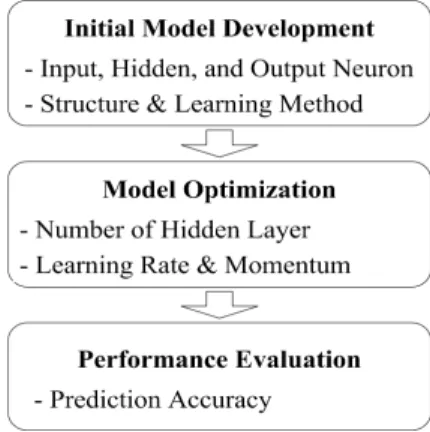
본 연구의 목적인 비재실기간 셋백온도에 따른 냉방부하 예측 모델 개발을 위한 과정은 크게 세 단계로 구성된다(그림 2). 첫 번 째 단계는 초기모델을 개발하는 것이다. 이 과정에서는 초기모 델의 입력층, 은닉층, 출력층 및 각 층 뉴런의 구성과 학습방법이 결정된다. 두 번째 단계는 개발된 초기모델을 최적화하는 것으 로써, 예측모델이 가장 안정적으로 결과값을 도출할 수 있는 은 닉층 수(NHL), 학습률(Learning Rate, LR), 그리고 모멘텀 (Momentum, MO)의 값을 결정하게 된다. 세 번째 단계는 최적 화된 모델의 성능분석을 실시하여 적용성을 확보하는 것으로써, 예측된 결과를 시뮬레이션된 결과와 비교하여 예측의 정확성 및 안정성이 분석된다.

Fig. 2. ANN model development process

2.1. 초기모델 개발

개발된 초기모델의 구성이 그림 3에 나타나 있다. 모델은 MATLAB을 사용하여 개발되었으며 각각 하나의 입력층, 은닉 층, 출력층으로 구성된다. 입력층은 9개의 뉴런으로 구성되어 있 다(TEMP_SETBACK, PERIOD_SETBACK, TEMP_{OA_nStep}, TEMP_{OA_}

AVE,nStep-60~nStep-1, TEMPOA_AVE,nStep-120~nStep-61, TEMP_{OA_AVE,}

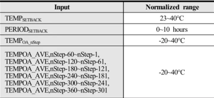
nStep-180~nStep-121, TEMPOA_AVE,nStep-240~nStep-181, TEMPOA_AVE, nStep-300~nStep-241, TEMPOA_AVE,nStep-360~nStep-301). 각 입력 값의 범 위는 표 1에 정리되어 있으며, 입력뉴런에 적용될 경우 식 (1)을 이용하여 0~1사이로 정규화 되어 사용된다. 출력층 뉴런의 수 (NHN)는 식(2)에 근거하여 19개로 구성되었다.^11,21)

출력뉴런은 셋백기간 중의 총냉방부하인 LOADSETBACK이다.

총냉방부하는 셋백기간 중의 냉방부하와 정상상태로 돌아오기 위한 냉방부하의 합으로 구성된다. 예를 들어 정상기간온도가 23°C, 셋백온도가 30°C로 각각 적용되었을 경우 총냉방부하는 셋백기간중 30°C를 유지하기 위한 냉방부하와 셋백기간 종료 후 정상기간온도인 23°C로 회복하기 위한 냉방부하의 합을 의 미한다. 즉, 셋백온도가 높을수록 셋백기간 중의 냉방부하는 감 소하는 반면 회복하기 위한 냉방부하는 증가하게 된다.

전이함수로는 Tanget-Simoid와 Pure-Linear 방식이 은닉층 뉴런과 출력층뉴런에 각각 사용되었다. 또한, 모델의 학습을 위 하여 Levenberg-Marquardt 알고리즘^1,21-23), 0.01 kWh의 goal, 1,000 times epoch, 0.6 LR, 그리고 0.4 MO²⁵⁾가 적용되었 다. 학습을 위하여 196세트의 학습데이터가 식 (3)에 근거하여 사용되었으며¹¹⁾, sliding-window method를 사용하여 데이터 세트를 유지하였다. 즉, 지속적 학습과정에서 가장 오래된 데이 터 세크는 새로이 획득되는 데이터세트에 의하여 대체된 후 학 습을 위하여 사용된다. 더불어 최적화 및 성능분석을 위하여 각 각 100 세트의 데이터가 별도로 준비되었다.

VAL_NOR = (VAL_ACT−VALMIN)/(VAL_MAX−VALMIN) (1)

NHN = 2NIN+1 (2)

ND = (NHN-(NIN+NON)/2)² (3)

Fig. 3. Initial model structure

(3)

Input Normalized range

TEMPSETBACK 23~40°C

PERIODSETBACK 0~10 hours

TEMPOA_nStep -20~40°C

TEMPOA_AVE,nStep-60~nStep-1, TEMPOA_AVE,nStep-120~nStep-61, TEMPOA_AVE,nStep-180~nStep-121, TEMPOA_AVE,nStep-240~nStep-181, TEMPOA_AVE,nStep-300~nStep-241, TEMPOA_AVE,nStep-360~nStep-301

-20~40°C Table 1. Normalization of the input variables

학습, 최적화 및 성능분석을 위한 데이터를 취득을 위하여 MATLAB (Matrix Laboratory)와 TRNSYS (Transient Systems Simulation) 소프트웨어를 함께 사용하였다. 그림 4는 데이터취득을 위하여 모델링된 테스트모듈을 보여준다. 데이터 세트는 6월 1일부터 9월 30일을 대상으로 셋백온도를 23°C에서 40°C 사이에서 변화시키면서 총냉방부하를 도출한 값으로 구성 하였다.

테스트모듈은 대한민국 서울에 위치한 것으로 가정하였으며 9개의 동일한 모듈 중 가운데에 위치하고 있다. 대상지역은 여름 철 고온다습한 기후적 특징을 가지고 있으며 6월에서 9월 사이 평균 23.5°C와 72.2%의 상대습도를 가진다.

모듈의 크기는 너비 3.6m, 높이 2.7m, 깊이 7.4m이며, 남쪽과 북쪽에 너비 2.0m, 높이 0.9m의 창이 하나씩 설치되어 있다. 건 물외피의 열저항은 외벽 2.801, 지붕, 바닥 0.491, 창문 0.353 m2K/W의 값으로 산정하였다. 침기 및 환기는 0.7 ACH의 비율 로 이루어지고 있으며, 실내부하는 착석하여 가벼운 일을 수행 하는 1인, 1대의 컴퓨터와 프린터, 5 W/m²의 조명발열로 이루어 진 것으로 가정하였다. 적용된 냉방시스템은 8,901 kJ/hr의 냉방 능력을 가지는 대류형 시스템이다.

그림 5는 테스트 모듈 모델링을 위하여 적용된 TRNSYS 요소 들의 구성을 보여주며 표 2에는 각 요소들의 기능이 정리되어 있 다. 테스트를 위하여 7 가지의 TRNSYS 타입이 사용되었다. 특 히, Type155는 TRNSYS와 MATLAB을 연결시켜주는 역할을 하여, TNRSYS에서 개발된 건물 모델과 MATLAB에서 개발된 인공신경망 모델의 연동이 가능하도록 하였다.

Fig. 4. Test module

Fig. 5. TRNSYS components

Types Roles

Type9c Calling a TMY2 weather file

Type16a Calculating the amount of solar radiation on building surfaces

Type69b Calculating the sky temperature Type33e Calculating the dew-point temperature Type56a-TR

NFlow

Calling the building model in the TRNBUILD Calculating the indoor temperature

Type155 Calling the algorithm in MATLAB Type65d-2 Producing and displaying the output file Table 2. Functions of the TRNSYS component types

2.2. 최적화 및 성능평가

모델의 예측성능과 안정성을 향상시키기 위하여 최적화 과정 이 진행되었다. 최적화 대상은 은닉층 수(NHL), 학습율(LR), 모 멘텀(MO)로 선정되었으며, 표 3에 정리된 바와 같이 일련의 대 상값에 대한 예측 비교 성능 분석이 실시되었다.

하나의 대상에 대한 성능 분석이 진행되는 동안 다른 변수는 일정 값으로 고정되었다. 예를 들어, 일련의 NHL에 대한 평가가 진행되는 동안 LR과 MO는 초기 설정값인 0.6과 0.4로 고정되 었다. 평가를 통하여 최적의 NHL 값이 결정되고난 후, LR에 대 한 평가가 이루어졌다. 이 경우 NHL과 MO는 각각 최적결정된 NHL값과 초기설정된 MO값으로 고정되었다. 동일한 방법으로 일련의 LR에 대한 예측 평가를 통하여 최적의 LR를 도출하였으 며, 최종적으로 최적 MO 선정으로 위한 평가 진행 시에는 NHL 과 LR은 앞 단계에서 결정된 최적값으로 고정시킨 후 평가를 진 행하였다.

최적값은 예측된 냉방부하(Si)와 시뮬레이션으로 구해진 냉방 부하(Mi)의 CVRMSE(Coefficient of Variation of the Root Mean Square Errors, %)가 가장 적은 경우를 의미하며(식 4), 이를 위해서 앞서 언급한 것과 같이 새로운 100세트의 데이터 세 트가 취득되었다.

마지막으로 최적화된 모델에 대한 최종 성능평가가 실시되었 다. 이를 위하여 새로운 100세트의 데이터가 사용되었다. 성능평 가를 위하여 Si와 Mi 간의 평균오차, 오차분포, 그리고 CVRMSE(%)가 분석되었다.

(4)

Components to be optimized

Parametric values to be tested

NHL 1 2 3 4 5 6 7 8 9 10

LR .1 .2 .3 .4 .5 .6 .7 .8 .9 1.0

MO .1 .2 .3 .4 .5 .6 .7 .8 .9 1.0

Table 3. Tested parametric values

_{  }



^^  





 ^

×  (4)

3. 결과 분석

모델 최적화의 결과가 표 4-6에 정리되어 있다. 첫 번째 단계 인 일련의 은닉층 수(NHL)에 대한 예측정확도 분석결과 Si와 Mi의 CVRMSE는 27.7%~76.0%까지 분포하는 것으로 나타났 으며, 최소의 경우는 3개의 NHL인 경우로 나타났다(표 4). 반 면, 초기 모델의 경우는 41.41%로써 최적 NHL 적용 시 예측 성 능이 현저히 향상되는 것으로 분석되었다. 따라서, 최적의 NHL 은 3으로 결정되었으며, 이 후 최적 LR, MO 선정을 위한 테스트 과정에서는 3개의 은닉층을 가진 모델로 평가되었다.

표 5는 일련의 학습률(LR)에 대한 예측성능 결과가 정리되어 있다. 0.1~1.0 사이의 LR 값을 가지는 모델에 대한 CVRMSE는 27.7%~42.3%로 나타났으며, 최소의 CVRMSE(27.7%)는 모 델의 학습률이 기본형인 0.6인 경우로 분석되었다. 따라서, 최적 의 모델은 0.6 LR로써 결정되었다.

일련의 MO에 대한 성능평가는 표 6에 정리되어 있다.

0.1~1.0 사이의 MO에 대한 CVRMSE는 22.8%~43.9%로 분 포되었으며, 최소의 CVRMSE(22.9%)는 MO 값이 0.2인 모델 인 경우 분석되었다.

위의 세 단계의 성능평가를 바탕으로 최적의 모델은 9 종류의 입력뉴런, 3-NHL, 1 종류의 출력뉴런, 0.6-LR, 그리고 0.2-MO의 구조와 학습방법을 가지도록 결정되었으며, 최종 모 델은 그림 6에 나타나 있다.

NHL

1 2 3 4 5 6 7 8 9 10

CVRMSE(%) 41.1 36.7 27.7 30.1 49.3 47.9 70.7 75.5 58.4 76.0 Table 4. Normalization of the input variables

LR

.1 .2 .3 .4 .5 .6 .7 .8 .9 1.0

MO

.1 .2 .3 .4 .5 .6 .7 .8 .9 1.0

Fig. 6. Optimized model

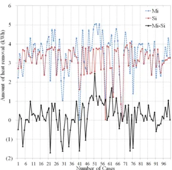
그림 7에는 셋백기간 중의 제거된 부하에 대한 예측 및 시뮬레 이션결과와 차이가 정리되어 있다. 총 100일의 결과가 비교되어 있으며, 예측결과와 시뮬레이션결과는 각각 0.00~5.05 kWh와 0.03~4.06 kW에 분포하고 있다. 특히, 표 7에는 Mi와 Si의 차이 분포가 정리되어 있다. 최적화된 모델의 예측 성능평가 결과(Si) 는 시뮬레이션 결과(Mi)와 하루 평균 0.58 kWh의 차이를 보이 는 것으로 분석되으며, 그 범위는 최소 0.01에서 2.47 kWh였다.

100개의 테스트 세트에 대하여 중 54 세트가 –0.5~0.5 kWh의 차이를 보이고 있고, 94 세트가 -1.5~1.5 kWh에 분포하고 있 다. 즉, 대부분의 경우 차이가 크지 않은 것으로 사료된다.

또한, 21.3%의 CVRMSE 결과를 나타내었으며, 이는 ASHRAE (American Society of Heating, Refrigeration and Air Conditioning) Guideline 14에서 제시한 기준인 CVRMSE 30% 보다 적은 값으로써 그 정확성이 확보되었다.²⁵⁾

Fig. 7. Profile of the Predicted and Simulated Results

(5)

Mi - Si

<=-1.5 <=-0.5 <=0.5 <=1.5 <=2.5

Number of Cases 4 9 54 30 3

Table 7. Error distribution

표 7에는 Mi와 Si의 차이 분포가 정리되어 있다. 최적화된 모 델의 예측 성능평가 결과(Si)는 시뮬레이션 결과(Mi)와 하루 평 균 0.58 kWh의 차이를 보이는 것으로 분석되으며, 그 범위는 최 소 0.01에서 2.47 kWh였다. 100개의 테스트 세트에 대하여 중 54 세트가 –0.5~0.5 kWh의 차이를 보이고 있고, 94 세트가 -1.5~1.5 kWh에 분포하고 있다. 즉, 대부분의 경우 차이가 크 지 않은 것으로 사료된다.

또한, 21.3%의 CVRMSE 결과를 나타내었으며, 이는 ASHRAE (American Society of Heating, Refrigeration and Air Conditioning) Guideline 14에서 제시한 기준인 CVRMSE 30% 보다 적은 값으로써 그 정확성이 확보되었다.²⁵⁾

4. 결론

본 논문은 비재실기간에 적용되는 셋백온도에 따른 냉방부하 예측을 위한 인공신경망기반 모델을 개발하는 것을 목적으로 하 였다. 개발의 과정은 초기모델개발, 모델 최적화, 그리고 성능평 가로 구성되었으며, 이를 위하여 시뮬레이션 데이터과의 비교를 실시하였다. 각 단계의 결과는 다음과 같이 정리된다.

(1) 초기 모델은 9개의 입력뉴런(TEMP_SETBACK, PERIOD

SETBACK, TEMPOA_nStep, TEMPOA_AVE,nStep-60~nStep-1, TEMPOA_

AVE,nStep-120~nStep-61, TEMPOA_AVE,nStep-180~nStep-121, TEMP_{OA_}

AVE,nStep-240~nStep-181, TEMPOA_AVE,nStep-300~nStep-241, TEMPOA_

AVE,nStep-360~nStep-301)으로 구성된 입력층, 19개의 뉴런으로 구성 된 한 층의 은닉층, 그리고 1개의 뉴런(LOADSETBACK)으로 구성 된 출력층으로 개발되었으며, 전이함수써 Tanget-Simoid와 Pure-Linear 방식이 은닉층뉴런과 출력층뉴런에 각각 사용되었 다. 또한, 학습을 위하여 Levenberg-Marquardt 알고리즘, 0.01 kWh의 goal, 1,000 times epoch, 0.6 LR, 그리고 0.4 MO가 적 용되었다.

(2) 이러한 초기 모델은 예측결과(Si)와 시뮬레이션결과(Mi) 의 최소화를 위한 최적화의 과정을 통하여 세개의 은닉층수와 0.6-LR, 0.2-MO의 학습방법을 가지도록 결정되었다.

(3) 최적화된 모델은 성능평가를 통하여 그 적용성을 테스트 하였으며, 그 결과 대부분의 경우에 대하여 Si와 Mi의 차이가 – 1.5에서 1.5 kWh 사이로 분석되었으며, CVRMSE 값이 21.3%

로써 일반적으로 적용가능한 기준인 30.0%보다 적은 것으로 분 석되어 가능성이 확보되었다.

본 연구에서 진행된 세 단계의 진행 결과 개발된 모델은 그 정 확성 및 안정성을 확보한 것으로 사료된다. 따라서, 개발된 모델 은 추후 제어알고리즘에 적용되어 최적 셋백온도의 결정과 건물

에너지 성능 향상을 가능하게 할 것으로 기대되며, 이를 위하여 추후 연구에서는 모델이 내재된 최적제어 알고리즘의 개발과 실 제 성능평가가 이루어져할 할 것으로 판단된다.

Acknowledgements

This research was supported by the Basic Science Research Program through the National Research Foundation (NRF) of Korea funded by the Ministry of Science, ICT & Future Planning (grant number 2015R1A1A1A05001142).

Reference

[1] J.W. Moon, J.J. Kim, ANN-based thermal control methods for residential buildings. Build. Environ. 2010, 45, 1612–1625.

[2] J.W. Moon, ANN-Based Model-Free Thermal Controls for Residential Buildings. Ph.D. Thesis, Taubman College of Architecture and Urban Planning, University of Michigan, Ann Arbor, MI, USA, 2009.

[3] W. McCulloch, W. Pitts, A logical calculus of ideas immanent in nervous activity. The Bull. Math. Biophys. 1943, 5, 115–

133.

[4] J.W. Moon, S.K. Jung, Y. Kim, S. Han, Comparative study of artificial intelligence-based building thermal control methods—

Application of fuzzy, adaptive neuro-fuzzy inference system, and artificial neural network. Appl. Therm. Eng. 2011, 31, 2422–2429.

[5] S.A. Kalogirou, C.C.Neocleous, C.N. Schizas, Building heating load estimation using artificial neural networks. In Proceedings of the International Conference CLIMA 2000, Brussels, Belgium, 30 August–2 September 1997; pp.1–8.

[6] K.W. Shin, Y.S. Lee, The study on cooling load forecast of an unit building using neural networks. Int. J. Air Cond. Refrig.

2003, 11, 170–177.

[7] S.H. Kim, B.S. Kim, Building load prediction using artificial neural networks in office renovation. In Proceeding of 3rd International Symposium on Architectural Interchanges in Asia.

The Architectural Institute of Korea, Cheju, Korea, 23–25 February 2000; pp. 604–612.

[8] D. Datta, S.A. Tassou, D. Marriott, Application of neural networks for the prediction of the energy consumption in a supermarket. In Proceedings of the International Conference CLIMA 2000, Brussels, Belgium, 30 August–2 September 1997;

pp. 98–107.

[9] S.A. Kalogirou, M. Bojic, Artificial neural networks for the prediction of the energy consumption of a passive solar building. Energy 2000, 25, 479–491.

[10] J.F. Kreider, X.A. Wang, D. Anderson, J. Dow, Expert systems, neural networks and artificial intelligence applications in commercial building HVAC operations. Autom. Constr. 1992, 1, 225–238.

[11] K.M. Aydinalp, V.I. Ugursal, Comparison of neural network, conditional demand analysis, and engineering approaches for modeling end use energy consumption in the residential sector.

Appl. Energy 2008, 85, 271–296.

[12] M. Aydinalp, V.I. Ugursal, A.S. Fung, Modeling of the space and domestic hot-water heating energy-consumption in the residential sector using neural network. Appl. Energy 2004, 79, 159–178.

[13] R. Platon, V.R. Dehkordi, J. Martel, Hourly prediction of a building's electricity consumption using case-based reasoning, artificial neural networks and principal component analysis.

Energy Build. 2015, 92, 10–18.

[14] R.Ž. Jovanović, A.A. Sretenović, B.D. Živković, Ensemble of various neural networks for prediction of heating energy consumption. Energy Build. 2015, 94, 189–199.

[15] B. Yuce, H. Li, Y. Rezgui, L. Petri, B.; Yang, C. Jayan,

(6)

Utilizing artificial neural network to predict energy consumption and thermal comfort level: An indoor swimming pool case study. Energy Build. 2014, 80, 45–56.

[16] S. Pandey, D.A. Hindoliya, R. Mod, Artificial neural networks for predicting indoor temperature using roof passive cooling techniques in buildings in different climatic conditions, Appl.

Soft Comput. 2012, 12, 1214–1226

[17] N. Morel, M. Bauer, M. El-Khoury, J. Krauss, Neurobat, a predictive and adaptive heating control system using artificial neural networks. Int. J. Sol. Energy 2001, 21, 161–201.

[18] A. Abbassi, L. Bahar, Application of neural network for the modeling and control of evaporative condenser cooling load.

Appl. Therm. Eng. 2005, 25, 3176–3186.

[19] A. Marvuglia, A. Messineo, G. Nicolosi, Coupling a neural network temperature predictor and a fuzzy logic controller to perform thermal comfort regulation in an office building. Build.

Environ. 2014, 72, 287–299.

[20] M. Mohanraj, S. Jayaraj, C. Muraleedharan, Applications of artificial neural networks for refrigeration, air-conditioning and heat pump systems—A review. Renew. Sustain. Energy Reviews 2012, 16, 1340–1358.

[21] J.W. Moon, J.H. Lee, Y. Yoon, S. Kim, Determining optimum control of double skin envelope for indoor thermal environment based on artificial neural network. Energy Build. 2014, 69, 175 –183.

[22] J.W. Moon, Performance of ANN based predictive and adaptive thermal control methods for disturbances in and around residential buildings. Build. Environ. 2011, 48, 15–26.

[23] Y.K. Baik. J.W. Moon, Development and performance evaluation of optimal control logics for the two position and variableheating systems in double skin façade buildings. The Int. J. Korea Inst. Ecol. Archit. Environ. 2014, 14, 71–77.

[24] J. Yang, H. Rivard, R. Zmeureanu, Online building energy prediction using adaptive artificial neural networks. Energy Build. 2005, 37, 1250–1259.

[25] American Society of Heating, Refrigerating, and Air-Conditioning Engineer. ASHRAE Guideline14-Measurement of energy and demand savings. ASHRAE Inc.; 2002.

Nomenclature

ANN: artificial neural network TEMP_SETBACK: setback temperature, °C

PERIOD_SETBACK: setback period during the daytime, minutes TEMPOA_nStep: outdoor air temperature in the current control cycle, °C

TEMPOA_AVE,nStep-60~nStep-1: average outdoor air temperature from nStep-60 to nStep-1, °C

LOAD_SETBACK: predicted amount of cooling load during the setback period, kWh

NIN: number of neurons in the input layer NHN: number of neurons in the hidden layer NON: number of neurons in the output layer NHL: number of hidden layer

LR: learning rate MO: moment

VALNOR: normalized value

VALACT: actual value of each input variable VAL_MIN: minimal value of each input variable VALMAX: maximal value of each input variable ND: number of datasets

Si: value predicted by the ANN model Mi: numerically simulated value Mavr: average of Mi