AOP를 이용한 유한체 위에서의 고속 병렬연산기의 구조
김용태*
An Architecture of the Fast Parallel Multiplier over Finite Fields using AOP
Yong-Tae Kim*
요 약
본 논문에서는 m은 홀수이고 n=mk인 경우에, 확대체 위에서의 곱셈기를 보조기로 사용하는 타입 k
가우스 주기를 가지는 유한 부분체 위에서의 새로운 병렬 곱셈기를 제안한다. 이 곱셈기의 공간과
시간 복잡도는 타입 IV인 경우에는 지금까지 알려진 곱셈기 중에서 가장 효율적인 Reyhani-Masoleh and Hasan의 곱셈기와 동등하다.
ABSTRACT
In this paper, we restrict the case as m odd, n=mk, and propose and explicitly exhibit the architecture of a new parallel multiplier over the field with a type k Gaussian period which is a subfield of the field implements multiplication using the parallel multiplier over the extension field . The complexity of the time and area of our multiplier is the same as that of Reyhani-Masoleh and Hasan’s multiplier which is the most efficient among the known multipliers in the case of type IV.
키워드
AOP(All One Polynomial), finite field, parallel multiplier.
AOP(모든 계수가 1인 다항식), 유한체, 병렬곱셈기
* 교육대학교 수학교육과 교수([email protected])
접수일자 : 2011. 10. 20 심사(수정)일자 : 2011. 12. 05 게재확정일자 : 2011. 12. 22 I. Introduction
Recently, finite fields are applied to areas such as Elliptic curve cryptosystem, XTR and ElGamal cryptosystem et al. In hardware implementation, it is well-known that finite fields with type I optimal normal bases generated by irreducible AOP(All One Poly- nomial) are the most efficient[1,2,3]. Since Massey-
Omura proposed the parallel multiplier over finite fields, Reyhani-Masoleh and Hasan[1] proposed the improved multiplier over finite fields in 2002 and then constructed the efficient multiplier over finite fields with type I optimal normal bases reducing the number of AND gates in 2003[2]. It also is well-known that if 8 cannot divide m, then there always exists a type k Gaussian normal basis by IEEE P1363[4,5], and for all m, the
finite field satisfies the condition
, the cyclic group generated by 2. Therefore we, in this paper, restrict the case as m odd, n=mk, and propose and explicitly exhibit the architecture of a new parallel multiplier over the field
with a type k Gaussian period which is a subfield of the field implements multiplication using the parallel multiplier over the extension field
. The complexity of the time and area of our multiplier is the same as that of Reyhani-Masoleh and Hasan’s multiplier[1,2] which is the most efficient among the known multipliers in the case of type IV.
II. Finite Fields
We, in this chapter, revisit properties of finite fields briefly. For any positive integer , there always exists a normal basis of over
[6,7]. That is, there exists ∊ such
that ⋯ is a normal basis of
over . Then is called a generator of the normal basis and, any ∊ is represented with respect to the normal basis by
∈and usually is represented by the coordinate system o
× ×
where [ ⋯ ]by vector form and T is the transposition of a matrix. One of the merits of normal basis is that the squaring an element
∈ is the only one Right Cyclic Shift(RCS) of the coordinate of . That is,
⋯ .
For ∊, the processes of the
computation of and the following theorem can be found in Gao et al.[7,8].
Theorem 1. ≧ , where is the number of non-zero entry of the multiplication matrix. So, any element of finite fields, in this paper, always is represented with respect to a normal basis.
1. Gaussian normal bases
Let m, k be positive integers, p = mk +1 ≠ 2 prime, e the order of 2 in , (mk/e, m) = 1 and the n-th primitive root of , the k-th root of unity and , then is the generator of the normal basis of
[6,7]. That is, is a normal basis of over . Then is called the Gaussian period of the type (m, k) over
[4,8] and we, in this paper, call of type k in this case. In Theorem 1, if , the normal basis N is said to be optimal. It is well-known that Gaussian normal bases of type k=
1, 2 satisfies the condition [7,9]. Then Gaussian normal basis is called type I optimal if k=1 and type II optimal if k=2[10]. The polynomial
having all coefficients 1 is said AOP. Following theorems are important in this paper.
Theorem 2. (Type I optimal normal basis)
has a type I optimal normal basis over
if and only if n+1 is prime and
or a root of the irreducible AOP
is the generator of the optimal normal basis[8,9,10].
Theorem 3. (Type II optimal normal basis) If 2m+1 is prime and or
≡ mod and , then
is the generator of the optimal normal basis of over , where is a primitive root of 2m+1[8,9,10].
2. Extension fields
Let n=mk, then is a subfield of . By the fundamental property of the finite field, for
∊ , ∊ if and only if . For brevity, we represent an element ∊ by coordinate system
∊ from now on. Then we have the following.
Theorem 4. Let ∊. Then ∊ if and only if for ≦
and ≡ , , that is,
⋯ .
Let m be odd, n = mk, n+1 primes and
in this paper. If is a (n+1)-th primitive root, then is the generator of the type I optimal normal basis of by Theorem 2 and (m, k) is the Gaussian period of
, since e = mk and = , and
is the generator of the normal basis of over . Thus A
∊ can be represented by
,
∊ .
Since is a subfield of , we have
∊. If
∊, then
, ≦ ≦ ≦ ≦ (1)
III. The Multiplier of Reyhani-Masoleh and Hasan using AOP
We, in this chapter, introduce the parallel multiplier over finite fields of Reyhani-Masoleh and Hasan using AOP[1,2]. We firstly transform the method for the computation of in as follows. In 2002, Reyhani-Masoleh and Hasan divided the matrix consisting of the basis matrix multiplication into
,
⋯
⋯
⋮ ⋮ ⋱ ⋮ ⋮
⋯
⋯
,
⋯
⋯
⋮ ⋮ ⋱ ⋮ ⋮
⋯
⋯
and proved the following theorem using the property that if ⋯ , then any element of U can be represented by
⋯ , and then proposed the parallel multiplier[1, Fig.1] by the theorem.
Theorem 5. Let ∊, then
⊙
⊙
,where are coordinates of A, B respectively,
⊙ ⊕ ⊙ , ⊕ XOR operator, ⊙ AND operator and all the indices are calculated modulo .
Let be generated by the irreducible AOP
⋯ and be a root of the AOP, then generates a type I optimal normal basis for
. In this case, for ⋯ , we have and in Theorem 5 since n is even. We thus have the following lemma usingthe fact that is a root of the AOP, and construct the Reyhani-Masoleh and Hasan’s multiplier[Fig. 1]
using the lemma and type I optimal normal basis.
Lemma 1.
⋯
,where satisfies the congruence
≡ . Let A, B∊, then
,
and if
⋯ ,
then we have the following lemma using for a multiplier.
Lemma 2. Let be a finite field with type I optimal normal basis and be a generator of the basis and ∊ , then
⊙≪ ≫
, ⊙≪ ≫⊕ ≪ ≫⊙,
where ≪ ≫= .
Fig. 1 RR-MO multiplier.
1. Multiplier reduced AND operations
In 2003, using the property that the multiplication matrix M is consisted of
⋯ ⋯ , for
≦ ≦ , Reyhani-Masoleh and Hasan[2]
proposed the parallel multiplier which can reduce the number of AND operation based on the following theorem. [2, Algorithm 1].
Theorem 6. Let ∊and . Then we have
⊙
⊙
,
⊕ ⊙ ⊕ ≦ ≦
≦ ≦ and all the indices are calculated modulo [2]. Reyhani-Masoleh and Hasan revised their algorithm[2, Algorithm 1] by applying to the type I optimal normal basis using Theorem 6 to gain the following algorithm.
Algorithm 1 (Low Complexity ONB-I Multi- plication over , [2])
Input : ∊ ≦ Output : C = AB
1. Generate ⊕≪ ≫⊙ ⊕≪ ≫ , ≦ , ≦ ≦ .
2. Generate
⊕≪ ≫⊙ ⊕≪ ≫,
≦ ≦ .
3. Initialize ≦ ≦
∊
4. For i =1 to v-1 { 5. ≦ ≦
⋯ . 6. R : = .
7. C : = C + R . 8. f : = f + . 9. }
10. If f is 1, C : = C + ( 1, 1, ... , 1 ).
11. }
In this algorithm, is that of Lemma 1.
IV. Multiplier over finite fields with type IV Gaussian normal Basis.
As above, we considered elements A, B of
as elements of the extension field with type I optimal normal basis and apply them to the multiplier of Chapter III to construct a new multiplier implementing the multiplication of A, and B efficiently.
Definition 1. Let n=mk and n+1 be primes,
and that of Lemma 1. If for ≦ ≦ ,
∊ , then we define as follows.
≡
≡
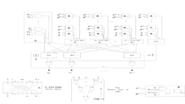
1. Architecture of the proposed multiplier For A, B ∊ ⊂, we now
calculate the complexity of Reyhani-Masoleh and Hasan’s multiplier proposed in 2002. The multiplier in chapter III first calculate only
⊙ ≦ ≦ instead of
⊙ ⊙ ≦ ≦ by the equation (2).
Secondly, we now calculate the values of
⊙≪ ≫⊕ ≪ ≫⊙from inputs
to using ≪ ≫ by the equation (1) of chapter II section 2.
1) For i = 1,
that is ⊙≪ ≫⊕ ≪ ≫⊕
≦ ≦ , by the equation (1) of chapter II section 2, we have
⊙⊕⊙ ⊙⊕⊙
⊙⊕⊙ ⊙⊕⊙
⋮
⊙⊕⊙
⊙⊕⊙
⊙ ⊕ ⊙
⊙⊕⊙ .
Then we have in general case
⊙
⊕ ⊙
⊙ ⊕⊙
≦ ≦ ≦ ≦
2) For i = 2, ... , u=(m-1)/2 ,
⊙≪ ≫⊕ ≪ ≫⊙
⊙ ⊕ ⊙,
≦ ≦ ≦ ≦ ,
≦ ≦ , and
⊙≪ ≫
⊕≪ ≫⊙
⊙ ⊕ ⊙ .
3) For i = u+1, ... m-1, i=u+s ,
≦ ≦ ,
≦ ≦ ≦ ≦ , we have
⊙ ⊕ ⊙
⊙ ⊕ ⊙
⊙⊕ ⊙
,
Since ≦ ≦ , is calculated by , ≦ ≦ in cases 1) and 2).
4) For ≦ ≦ ,
⊙≪ ≫⊕ ≪ ≫⊙
⊙ ⊕ ⊙ .
⊙ ⊕ ⊙
⊙ ⊕ ⊙
⊙⊕ ⊙
.
Since ≦ ≦ , is calculated by , ≦ ≦ in cases 1) and 2).
5) For i = m+1, ..., (k/2)m –1,
≠ , , ≦ ≦
≦ ≦ ,
⊙≪ ≫ ⊕≪ ≫⊙
⊙ ⊕ ⊙
.
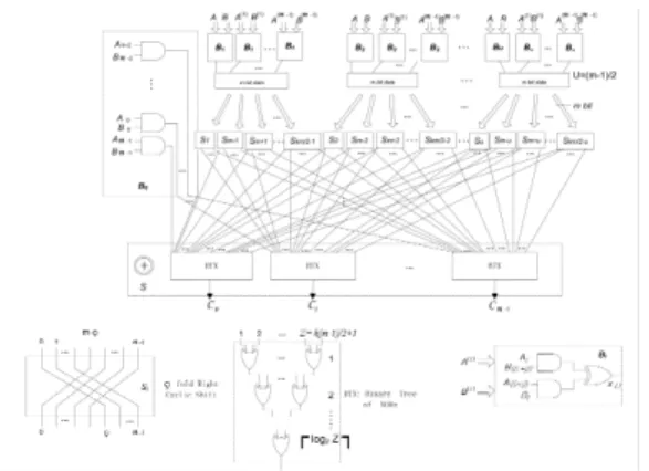
Here for ≦ ≦ , blocks
are
obtained by rewiring the block
. That is, for
≦ ≦ , blocks
are inputted according to the order of calculating blocks
. , ≦ ≦ , however, are inputted by shifting, since
⊙≪ ≫⊕ ≪ ≫⊙
≪ ≫⊙⊕ ⊙≪ ≫
,
.
Since values of blocks , in this stage, are all 0, we need not calculate them.
For ≦ , Reyhani-Masoleh and Hasan’s multiplier in chapter III is implemented at the block through the block by RCS satisfying of Lemma 1. Since, on the other hand,
∊ ⊂and ∊, m coordinates are represented by k repetitions so that we calculate coordinates from 0-th to (m-1)-th as chapter II section 2. Thus for blocks
≦ ≦ , the outputs of blocks from blocks
, ∊ , are obtained by RCSs. All the properties discussed above lead the following. Theorem 7. Let be with type (m, k) Gaussian period, n = mk,
. If
∊ ⊂ and C=AB then we have
,
⊙
⊕
⊙
≦ ≦ ≦