Design of Extended Terminal Sliding Mode Control Systems

(1)

DOI:10.5302/J.ICROS.2011.17.3.236 ISSN:1976-5622 eISSN:2233-4335

I. 서론

. (state space)

(sliding surface) ,

[1-3].

1 (linear combination) .

(exponentially stable) 0

,

. Zhihong

0

4], Park

[5].

[6,7].

.

, 0

1

( ) ,

0 1

. DC

motor .

* (Corresponding Author)

: 2010. 12. 19., : 2010. 12. 27., : 2010. 12. 30.

, , :

([email protected]/[email protected]/[email protected])

문제 정의 II.

(canonical form)

2 .

   (1)

  ^∈^, ∈, 



 ^



 

_ _ , 



 ^





_ .

.

    ^. (2)

 ,  (signum

function) ,       .

(3) ,

     

[5-7].

    ^. (3)

.

제어기 설계 III.

, ,

0 .

정리 1: ,

    , 0

(relaxation time, _) .

_   

^{  }

 (4)

증명:      ≧  , (2) .

Design of Extended Terminal Sliding Mode Control Systems

, , ^*

(Young-Hun Jo¹, Yong-Hwa Lee¹, and Kang-Bak Park¹)

1Korea University

Abstract: The terminal sliding mode control schemes have been studied a lot since they can guarantee that the state error gets to zero in a finite time. However, the conventional terminal sliding surfaces have been designed using power function whose exponent is a rational number between 0 and 1, and whose numerator and denominator should be odd integers. It is clearly restrictive. Thus, in this paper, we propose a novel terminal sliding surface using power function whose exponent can be a real number between 0 and 1.

Keywords: terminal sliding surface, SMC (Sliding Mode Control), nonlinear control

(2)

^ . (5)

 0 (relaxation time) _

, .



  ^

⇔ ^

   

⇔ _^^^^{ }^{  }_^^^

⇔   

^{  }



_^^^{   }^^

(6)

_   , .

  

^{  }



_^^^{   }^

⇔    

^{  }

   _

⇔ _   

^{  }



(7)

      , (2) .

  ^ . (8)

(8) (6)~(7)

.

_   

 ^{  }

 (9)

(7) (9) .

_   

^{  }

 (10)

(10) ,

. .

정리 2: (1) ,

0 .

  ^{ }  _ ^{  } _

 ^^{  }  _^ (11)

_ _ .

증명: .

_{ }



^. (12)

 ≧  , .

 

 ^{  }

 ^  _ ^{  }^

(13)

 ≧  , (2) .

    ^ ⇔     ^. (14)

(14)  (13) ,

.

 ^  __  ^{  }

 ^  __  ^{  }  ^

 ^  _^{  } ^^{  } _^

(15)

  

.

 

  ^{  }

 ^  __   ^{  }

 ^  __

  ^{  }   ^

 ^  _ ^{  }

 ^ ^{  } _^

(16)

(15) (16)  (11)

.

    _^ _ (17)

(17) _ _ ,  0

(_{}) .

_{}≦ _



(18)

. (12)  (positive

definite function) , (17)  (negative definite function) (  )

(  ) .

1

0 .

(singular point) .

.

   ^ ^{    } (19)

(3)

실험 결과 IV.

DC

(_ , _ , _ ) . DSP

, 1msec. ,

  , _ , _  .

, (3)

 0 1

[5-7].

,

.  ,

짝수

홀수 , 홀수

짝수 .

1~4  ,   ^



. 1 ,

0 .

2 

. ,

,

.

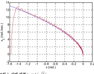
3 , 4

0 0.2 0.4 0.6 0.8 1

-1.6 -1.4 -1.2 -1 -0.8 -0.6 -0.4 -0.2 0 0.2

Time (sec.)

Output (rad.)

1. () (  ^).

Fig. 1. The output () (  ^).

0 0.2 0.4 0.6 0.8 1

-14 -12 -10 -8 -6 -4 -2 0 2

Time (sec.)

sliding variable ( s)

2. () (  ^).

Fig. 2. The sliding variable () (  ^).

-1.6 -1.4 -1.2 -1 -0.8 -0.6 -0.4 -0.2 0 0.2 -2

0 2 4 6 8 10 12 14

x (rad.) x 2 (rad./sec.)

3. (  ^).

Fig. 3. The phase portrait (  ^).

0 0.2 0.4 0.6 0.8 1

-5 0 5 10 15 20 25

Time (sec.)

Input ( u)

4. () (  ^).

Fig. 4. The input () (  ^).

0 0.2 0.4 0.6 0.8 1

-1.6 -1.4 -1.2 -1 -0.8 -0.6 -0.4 -0.2 0 0.2

Time (sec.)

Output (rad.)

5. () (  ).

Fig. 5. The output () (  ).

(4)

.

5~6  짝수

홀수 ,   



. 5 ,

, 0

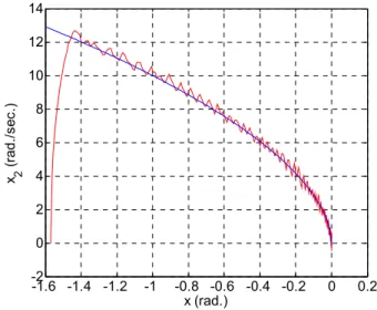
. 6

.

7~8  홀수

짝수 ,   



. 7 ,

, 0

. 8

.

,

0 1

.

-1.6 -1.4 -1.2 -1 -0.8 -0.6 -0.4 -0.2 0 0.2 -2

0 2 4 6 8 10 12 14

8. () (  ).

Fig. 8. The output () (  ).

V. 결론

. ,

, 0 1

,

0 1 .

.

참고문헌

[1] V. I. Utkin, “Variable structure systems with sliding mode,” IEEE Trans. on Automatic Control, vol. 22, no.

2, pp. 212-222, Apr. 1977.

[2] J. Y. Hung, W. Gao, and J. C. Hung, “Variable struc- ture control: a survey,” IEEE Trans. on Industrial Electronics, vol. 40, no. 1, pp. 2-22, Feb. 1993.

[3] C. Edwards and S. K. Spurgeon, Sliding Mode Control, Taylor & Francis Ltd, 1998.

[4] M. Zhihong, A. P. Paplinski, and H. R. Wu, “A robust terminal sliding mode control scheme for rigid robotic manipulators,” IEEE Trans. on Automatic Control, vol.

39, no. 12, pp. 2464-2469, Dec. 1994.

[5] K. B. Park and J. J. Lee, “Comments on a robust terminal sliding mode control scheme for rigid robotic manip- ulators,” IEEE Trans. on Automatic Control, vol. 41, no.

5, pp. 761-762, May 1996.

[6] L. Wang, T. Chai, and L. Zhai, “Neural-network based terminal sliding-mode control of robotic manipulators in- cluding actuator dynamics,” IEEE Trans. on Industrial Electronics, vol. 56, no. 9, pp. 3296-3304, Sep. 2009.

[7] Y. Feng, J. Zheng, X. Yu, and N. V. Truong, “Hybrid terminal sliding-mode observer design method for a per- manent-magnet synchronous motor control system,” IEEE Trans. on Industrial Electronics, vol. 56, no. 9, pp.

3424-3431, Sep. 2009.

-1.6 -1.4 -1.2 -1 -0.8 -0.6 -0.4 -0.2 0 0.2 -2

0 2 4 6 8 10 12 14

6. (  ).

Fig. 6. The phase portrait (  ).

0 0.2 0.4 0.6 0.8 1

-1.6 -1.4 -1.2 -1 -0.8 -0.6 -0.4 -0.2 0 0.2

Time (sec.)

Output (rad.)

7. () (  ).

Fig. 7. The output () (  ).

(5)

2009 . 2009 ~

.

, .

1990 (

). 1992 (KAIST)

( ). 1997

. 1997 ~1999 2 . 1997 12 ~

1999 2 (KIT)

. 1999 3 ~ .

, , ,

.

2010 . 2010 ~

.

, .