In-plane Vibration Analysis of Rotating Cantilever Curved Beams

(1)

In-plane Vibration Analysis of Rotating Cantilever Curved Beams

Guang Hui Zhang * , Zhan Sheng Liu ** and Hong Hee Yoo

^†

Key Words : Curved beam(굽은보), In-plane vibration(면내 진동), Rotating(회전), Stiffness variation(강성변화), Dimensionless parameter(무차원 매개변수)

Abstract

Equations of motion of rotating cantilever curved beams are derived based on a dynamic modeling method developed in this paper. The Kane’s method is employed to derive the equations of motion. Different from the classical linear modeling method which employs two cylindrical deformation variables, the present modeling method employs a non-cylindrical variable along with a cylindrical variable to describe the elastic deformation. The derived equations (governing the stretching and the bending motions) are coupled but linear. So they can be directly used for the vibration analysis.

The coupling effect between the stretching and the bending motions which could not be considered in the conventional modeling method is considered in this modeling method. The natural frequencies of the rotating curved beams versus the rotating speed are calculated for various radii of curvature and hub radius ratios.

Symbols

ρ

: mass per unit length of beam

i i q

q₁, ₂ : generalized coordinates

vrP: velocity of generic point P arP: acceleration of generic point P

vrO: velocity of point O fixed to the rigid hub

ω

^rA: angular velocity of the rigid hub

rr : vector from O to P ur : vector from P to P′

r : radius of the rigid hub

1. Introduction

Curved beam structures can be found in many aerospace and mechanical engineering examples such as spacecraft structures, robots, turbine blades, and helicopter blades. For proper designs of such systems, their modal characteristics such as natural frequencies should be accurately identified. Although most of the previous studies dealt with straight beams, a few researchers investigated the modal characteristics of curved beams. Compared with the modal characteristics of straight beams, those of curved beams show clearly

different characteristics that are originated from the curvature of curved beams. Furthermore, the modal characteristics of rotating curved beams are significantly different from those of non-rotating curved beams. The variation results from the stretching caused by centrifugal inertia force due to rotational motion. The stretching as well as the curvature variation causes the increment of the bending stiffness of the structures, which will naturally result in the variation of natural frequencies.

An analytical method to calculate the natural frequency of a rotating beam was originally introduced by Southwell and Gough[1]. Based on the Rayleigh energy method, they proposed an equation to calculate the natural frequencies of rotating cantilever beams. To obtain more accurate results, Schilhansl[2] derived a linear partial differential equation which governs the bending vibration of a rotating beam. Putter and Manor[3] applied the assumed mode approximation method for the modal analysis of a rotating beam. More recently, Kane et al. [4] introduced a comprehensive theory to deal with the dynamics of a beam attached to a base. A new variable, namely the stretch along the elastic axis, is used to account for geometric nonlinearity appropriately. Based on the method, the effect of Coriolis coupling on the modal characteristics of a rotating beam was successfully investigated by Yoo and Shin[5].

The out-of-plane and the in-plane motions of a curved beam are coupled in general. However, if the cross section of the curved beam is symmetric and the thickness of the beam is small in comparison with the radius of the beam, the out-of-plane and the in-plane motion can be decoupled[6, 7]. The Rayleigh-Ritz method could be used to obtain the natural frequencies of inextensional [8, 9] and extensional [10, 11] in-plane vibrations of ring segments.

Upper and lower bounds for the fundamental frequency of in-

† School of Mechanical Engineering, Hanyang University E-mail : [email protected]

TEL : (02)2220-0446 FAX : (02)2293-5070

*

School of Mechanical Engineering, Hanyang University

**

School of Energy Science and Engineering, Harbin Institute of Technology, China

(2)

plane transverse vibration of cantilever curved beam were determined by Laura[12]. Laura derived the fundamental natural frequency equation by means of the Rayleigh-Ritz method. Three curved beam elements were investigated to solve the problem of radial vibrations of curved beams [13].

The purpose of this paper is to develop a modeling method to investigate the modal characteristics of a rotating cantilever curved beams. For the modeling method a hybrid set of deformation variables are employed. The use of hybrid deformation variables, which distinguishes the present modeling method from other conventional method, is the key ingredient to derive accurate linear equations of motion. The linear equations provide proper motion induced stiffness variation.

Moreover, the coupling effect between the stretching and the bending motion could be considered in the equations. The effects of the curvature along with the hub radius and the rotating speed on the modal characteristics of curved beams are investigated with numerical examples.

2. Equations of motion

2.1 Assumption and geometric constraint equation In this section, equations of motion of a rotating cantilever curved beam are derived based on the following assumptions.

The beam has homogeneous and isotropic material properties.

The elastic and the centroidal axes of the cross-section of a beam coincide so that effects due to eccentricity need not be considered. The beam has a slender shape so that the shear and the rotary inertia effects can be neglected. The shear strains due to change of normal stresses, such as bending and warping normal stresses, are negligibly small (Euler- Bernoulli hypothesis). These assumptions result in simplified equations of motion with which the main issues of this study (the stiffening effect and modal characteristics variation due to rotation) can be effectively investigated.

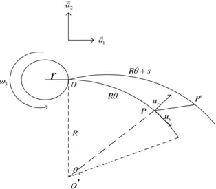
Fig.1 shows the configuration of a rotating curved beam attached to a hub. A generic point P which lies on the undeformed neutral axis moves to P′ when the beam is deformed. Cylindrical deformation variables u_r

and u_θ are conventionally employed to express the elastic deformation. In the present study, a non-cylindrical variable s denoting the stretch along the neutral axis of the beam is employed instead of u_θ .

There is a geometric relation between the stretch s and the cylindrical deformation variables. This relation is later used to drive the generalized inertia forces. From the differential geometry (see Ref.[15]), the following equation can be obtained.

1

2 2 2

0

u ur

OP ^θ R ^θ dσ

σ σ

⎡⎛ ∂ ⎞ ⎛∂ ⎞ ⎤

′ =

∫

⎢⎢⎣⎜⎝ +∂ ⎟⎠ +⎜⎝∂ ⎟⎠ ⎥⎥⎦ (1)

where OP′ denotes the length of the curved beam after deformation. If the stretch variable s is employed, one can write the equation as follows:

r

o

o′

R ar2

ar1

θ0

P Rθ P′

Rθ+s

ur

u_θ ω3

Fig. 1 Configuration of a rotating cantilever curved beam

1

2 2 2

0

u ur

Rθ s ^θ R ^θ dσ

σ σ

⎡⎛ ∂ ⎞ ⎛∂ ⎞ ⎤

+ =

∫

⎢⎢⎣⎜⎝ +∂ ⎟⎠ +⎜⎝∂ ⎟⎠ ⎥⎥⎦ ₍₂₎ By using binomial expansion of the integrand of equation (2), the following approximated equation can be obtained.

2

0

1 2

ur

s u d

R

θ

θ σ

σ

⎛∂ ⎞

= +

∫

⎜⎝∂ ⎟⎠ (3)

2.2 Approximation of deformation variables and strain energy expression

In the present work, s and u_r are approximated by using functions and corresponding coordinates to drive the ordinary differential equations of motion. The modeling method employing hybrid deformation variables is described in detail in Ref.[5]. By employing the Rayleigh-Ritz method, the deformation variables are approximated as follows:

¹ 1( ) ( )1 1

i i

i

s q t

μ θ

=

∑

Φ (4)

( ) ( )

2

2 2

1

r i i

i

u q t

μ θ

=

∑

Φ (5)

where _Φ_1i and _Φ_2i are the spatial function for s and

ur ;

μ

₁ and

μ

₂ are the numbers of generalized coordinates q_1i and q_2i. Using the strain energy form (in Ref.[12]) employing the stretch variable s, the total strain energy can be described as follows:

0 0

2 2 2

3 2

0 0

1 1

2 2

r r

d u

ds EI

U EA d u d

R d R d

θ θ

⎛ ⎞

=

∫

⎜⎝ ⎟⎠ +

∫

⎜⎝ + ⎟⎠ ⁽⁶⁾

where E is Young’s modulus, A is the cross-section area, I is the second area moment of the cross-section, R is the radius of the curved beam, and θ is the curvature ₀ angle of curved beam. Thus, θ =0 at the fixed end and θ θ= ₀ at the free end.

(3)

2.3 Equations of motion

Under the assumptions given in Section 2.1, the equations of motion can be derived from the following equation (see Ref.[14]).

0

0 0

p p

i i

v U

R a d

q q

θ ρ ^⎛⎜⎝^∂∂ ^⎞⎟⎠ θ+^∂∂ =

∫

^r ^r_& (7)

The acceleration ar^p can be obtained by differentiating the velocity vr^p with respect to time, which can be obtained by using the following equation.

( ) ^A ( )

p o A d r u

v v r u

ω dt⁺

= + × + + r r

r

r r r r (8)

The third term in the right hand side of Eq. (8) denotes the time differentiation of vectorrr r+u in the frame A (the rigid hub). Using the coordinate systems fixed to the rigid hub, vr^o,

ω

^r^A, rr and urcan be expressed as follows:

3 2

vro=ωrar

(9)

3 3

A a

ωr =ω r

(10)

1 2

sin (1 cos )

rr=R θar −R − θ ar

(11)

(cos 2 sin 1) (cos 1 sin 2)

ur_θ =ur θar + θar +u_θ θar − θar

(12)

The velocity of point P can be obtained as follows

( )

[ ] [ ]

[ ]

3 3 3 1

1 3 3 2

3 3 2

1 cos cos sin

sin cos sin

cos cos sin sin

p

r r

v R u u a

u u a r R a

u u u u a

θ θ

ω θ ω θ ω θ

θ θ ω ω θ

ω θ θ θ ω θ

=⎡⎣ − − + ⎤⎦

+ + + +

+ + − +

r r

& &

& & r

(13)

Using Eqs. (3) and (13) , the partial derivative of the velocity of P with respect to the generalized speed q&_i can be obtained as:

( )

2

2 1 0 2 , 2 , 2 1

1

sin cos cos

u p

j j j i j

i j

v d q a

q R

θ

η η

θ θ θ η

=

∂∂^r_& =⎡⎣ Φ + Φ −

∑∫

Φ Φ ⎤⎥⎦^r

( )

2

2 1 0 2 , 2 , 2 2

1

cos sin sin

u

j j j i j

j

d q a R

θ

η η

θ θ θ η

=

⎡ ⎤

+⎣ Φ − Φ + Φ Φ ⎥

∑∫

⎦^r ⁽¹⁴⁾ where

η

denotes partial differentiation with respect to the dummy variable

η

. By differentiating Eq. (13) , the acceleration of P can be obtained as follows:

[

( )

[

( )

3 3

2 2 2

3 3 3 1

3 3

2 2 2

3 3 3 2

2 cos 2 sin sin cos

sin sin cos

2 sin 2 cos cos sin

1 cos cos sin

p

r r

r

r r

r

a u u u u

r R u u a

u u u u

R u u a

θ θ

θ

θ θ

θ

ω θ ω θ θ θ

ω θ ω θ ω θ

ω θ ω θ θ θ

ω θ ω θ ω θ

= − + + +

− + − − ⎤⎦

+ + + −

⎤

+ − − + ⎦

r & & && &&

r

& & && &&

r

(15)

By linearizing the generalized inertia forces, equations of motion are finally obtained as follows.

( ) ( )

( ) ⁽ ⁾

1

0 0

1 1 1 3 1 2 1

0 0

1

2

3 0 1 1 1 0 1 , 1 , 1

2 2 2

3 0 1 3 0 1

2 1

cos sin

j i j j i j

j

j i j j i j

j j

R d q R d q

R d q EA d q

R

R r d R d

μ θ θ

θ θ

ρ θ ω ρ θ

ω ρ θ θ

ω ρ θ θ ω ρ θ θ

=

⎡ Φ Φ + Φ Φ

⎢⎣

− Φ Φ + Φ Φ ⎤⎥⎦

= Φ + Φ

∑ ∫ ∫

∫ ∫

&& &

₍₁₆₎

( ) ( )

( )

{ }

( )

2 0 0

0 0

0

2 2 2 3 2 1 2

0 0

1

2

3 0 2 2 2 3 0 2 , 2 ,

2 , 2 2 , 2 2 2 2

3 0

2

3 0 0 2 , 2 , 2

2

3 0 2 ,

2 1 1

sin sin

cos cos

j i j j i j

j

j i j j i

j i i j j i j

j i j

j

R d q R d q

R d q EI d

R

EI d EI d EI d q

R

r d q

R

μ θ θ

θ θ

θθ θθ

θ

θθ θθ

θ

θ θ

θ

ρ θ ω ρ θ

ω ρ θ θ

θ θ θ

ω ρ θ θ θ

ω ρ θ θ

=

⎡ Φ Φ − Φ Φ

⎢⎣

− Φ Φ + Φ Φ

+ Φ Φ + Φ Φ + Φ Φ

− − Φ Φ

+ − Φ

∑ ∫ ∫

∫ ∫

∫

&& &

{

⁰

}

0 0

2 , 2

0

2 2 2

3 0 sin 2 3 0 cos 2

i j

j j

d q

R r d R d

θ

θ θ

θ

ω ρ θ θ ω ρ θ θ

Φ ⎤⎥⎦

= Φ − Φ

∫

∫ ∫

2 0 2

3 0^θ R 2jd

ω ρ θ

+

∫

Φ ₍₁₇₎ The underline terms indicate the stiffness variation induced by rotational motions.

2.4 Dimensionless equations of motion

To lend generality to the numerical results, Eqs.(16, 17) are transformed into dimensionless equations. Several dimensionless variables and parameters are defined as follows:

^t

τ T (18)

0

ξ θ

θ ₍₁₉₎

0 j j

q q

Rθ (20)

r

δ R ₍₂₁₎ T 3

γ ω (22)

4 4

R 0

T EI

ρ θ (23)

The parameters

γ

and δ represent the angular speed ratio and the hub radius ratio. For the modal analysis, the right hand terms of the equations can be ignored. Thus the dimensionless equations of motion are obtained as

1

11 21 2 11 2

1 1 1 1

1

2 ^S 0

ij j ij j ij j ij j

j

m q m q m q k q

μ

γ γ α

=

⎡ + − + ⎤=

⎣ ⎦

∑ ^&& ^& (24)

2

22 12 2 22 2 2

2 2 2 2 2 2

1

2 ^B ^GA ^GB 0

ij j ij j ij j ij j ij j ij j

j

m q m q m q k q k q k q

μ γ γ γ δ γ

=

⎡ − − + + + ⎤=

⎣ ⎦

∑ ^&& ^& ⁽²⁵⁾

where

1

ij 0 i j

m^αβ =

∫

ψ ψ_α _β dξ (26)

1 1 , 1 , 0 S

ij j i

k =

∫

ψ ψ_ξ _ξdξ (27)

1 1 1 1

2 2 4

2 , 2 , 0 2 , 2 0 2 , 2 0 2 2

0 0 0 0

B

ij j i j i i j j i

k =∫ψ ψ_ξξ _ξξdξ θ ψ ψ ξ θ ψ ψ ξ θ ψ ψ ξ+ ∫ _ξξ d + ∫ _ξξ d + ∫ d ⁽²⁸⁾

(4)

( ) ( )

1 0 0

2 , 2 ,

2 0

0

1 1 1 cos sin

2 2

GC

ij j i

k ξ θ ξ θ _ξ _ξd

ψ ψ ξ

θ

+ −

= ∫ (29)

( ) ( )

1 0 0

2 , 2 , 2 0

0

1 1 1 sin sin

2 2

GS

ij j i

k ξ θ ξ θ ψ ψ_ξ _ξdξ

θ

+ −

= ∫ (30)

where

ψ

is the function of

ξ

rather than θ. In Eq.(24), the α is defined as follows:

( ₀)² ^{1 2}

A R I α= ⎜^⎛⎜⎝ θ ^⎞⎟⎟⎠

(31)

This parameter which is often called the slenderness ratio is proportional to the length to thickness ratio of the beam.

2.5 Modal formulation

Eq. (24) and(25) are expressed in a matrix form as follows：

1

1 1

11 12 11

1

2 2

22 21 22

0 0 0

0 0 0 0

j

j j

j

j j

q

q q

M C K

q

q q

M C K

⎧ ⎫ ⎧ ⎫ ⎧ ⎫

⎡ ⎤⎪⎨ ⎪⎬+⎡ ⎤⎪⎨ ⎪⎬+⎡ ⎤⎨ ⎬=

⎢ ⎥⎪ ⎪ ⎢ ⎥⎪ ⎪ ⎢ ⎥

⎣ ⎦⎩ ⎭ ⎣ ⎦⎩ ⎭ ⎣ ⎦ ⎩ ⎭

&& &

&& & (32)

In Eq.(32), M₁₁and M₂₂ denote matrices which are composed of elements m¹¹_ij and m_ij²². The sub-matrices are defined as follows:

12 2 12

C = − γM (33)

21 2 21

C = + γM (34)

2 2

11 11 s

K = −γ M +α K (35)

2 2 2

22 22 B GA GB

K = −γ M +K +γ δK +γ K (36)

3. Numerical study and discussion

In Table 1, the first natural frequency of the non-rotating cantilevered curved beams obtained with the present modeling method are compared to those of Ref.[12] in which Rayleigh-Ritz method is employed to obtain the upper bound and the Dunkerley’s method is employed to obtain the lower bound. This shows that the present method is qualitatively equivalent to the conventional modeling method if the motion induced stiffness variation effect is ignored.

The natural frequencies of straight beam increase as the rotating speed increases. For curved beams with large radius and small curvature angle (almost straight beam) their natural frequencies increase as those of straight beams do.

However, when the curvature angle gets larger, the first natural frequency may decrease.

The first bending natural frequency variation is shown in Fig.2(a). To obtain the result, 8 assumed modes are used. When the curvature angle is small, the first bending natural frequency increases. But as the curvature angle increases, the increasing rate of the first natural frequency gets attenuated. The second natural frequency variation is shown in Fig.2(b). It exhibits the same increasing trends as that of the straight beam. As the rotating angular speed increases, the second bending natural frequency increases. When the curvature angle increases, the second bending natural frequency decreases.

Table 1 Comparison of the first bending natural frequency θ0 Upper bound

Ref.[12]

Lower bound Ref.[12]

Present

10 3.51 3.466 3.518 20 3.52 3.473 3.523 30 3.53 3.483 3.533 40 3.55 3.498 3.546 50 3.57 3.517 3.564 60 3.59 3.540 3.587 70 3.62 3.568 3.614 80 3.66 3.600 3.646 90 3.71 3.637 3.684

0.0 0.5 1.0 1.5 2.0 2.5 3.0

3.50 3.55 3.60 3.65 3.70 3.75

dimensionless first natural frequencies ( ω )

dimensionless angular speed ( γ ) θ0=5⁰

θ₀=30⁰ θ0=60⁰ θ₀=90⁰

(a)

0.0 0.5 1.0 1.5 2.0 2.5 3.0

21.6 21.8 22.0 22.2 22.4 22.6 22.8 23.0 23.2

dimensionless second natural frequencies (ω)

dimensionless angular speed ( γ )

θ0=5⁰ θ

0=30⁰ θ0=60⁰ θ₀=90⁰

(b)

Fig.2 Bending natural frequency variations (a) first natural frequency (b) second natural frequency

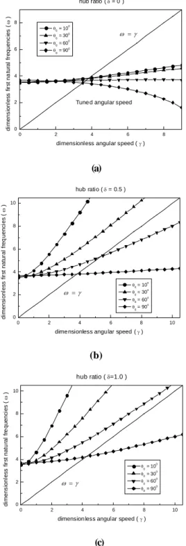
When the angular speed of a rotating cantilevered curved beam matches the natural frequency (as shown in Fig.3(a)), resonance may occur. Such an angular speed is usually called the tuned angular speed. Severe resonance phenomena may occur at the tuned angular speed during the operation of the rotating beams. So the tuned angular speed must be calculated for safe designs of rotating beams. The tuned angular speeds for different hub radius ratios are shown in Fig.3.

(5)

0 2 4 6 8 0

2 4 6 8

Tune d angular speed ω =γ hub ratio ( δ = 0 )

dimensionless angular speed ( γ ) θ₀ = 10⁰

θ0 = 30⁰ θ₀ = 60⁰ θ₀ = 90⁰

(a)

0 2 4 6 8 10

ω =γ

hub ratio ( δ = 0.5 )

dimensionless angular speed ( γ ) θ₀ = 10ô θ0 = 30ô θ₀ = 60ô θ0 = 90ô

(b)

0 2 4 6 8 10

ω=γ

hub ratio ( δ=1.0 )

dimension less angular speed ( γ ) θ0 = 10⁰ θ₀ = 30⁰ θ0 = 60⁰ θ₀ = 90⁰

(c)

Fig.3 Tuned angular speed in bending vibration with different hub ratiosσ. (a) σ =0 (b) σ =0.5 (c) σ =1

The above figures indicate that the curvature angle of a curved beam may significantly affect the tuned angular speed.

The case of zero hub radius ratio is shown in Fig.3(a). It is observed that the tuned angular speed varies with the curvature angle (from 0^o to 90^o). As the curvature angle increases, the tuned angular speed decreases. In Fig.3(b), it indicates that the curved beams with small curvature angle have no tuned angular speed if the hub radius ratio exceeds a certain

value. As the curvature angle exceeds 60^o the tuned angular speed exists. It means that resonance will not happen with a small curvature angle. Fig.3(c) shows that the tuned angular speed exists only if the curvature angle increases large enough. As the hub radius ratio increases, the tuned angular speed of certain curvature angle increases. Also the tuned angular speed of a beam with small curvature angle disappears when the hub radius ratio increases. If the curvature angle is equal to90^o, the tuned angular speed exists with a hub ratio (between 0 to 1).

0 20 40 60 80 100

0 50 100 150 200 250

1 B

2 B

3 B

1 S

δ=0.1 α=70 θ=10⁰

dimensionless natural frequencies ( ω )

dimensionless ang ular speed ( γ ) coupling considered coupling ignored

(a)

0 20 40 60 80 100

0 50 100 150 200 250

1 S

3 B

2 B

1 B

δ=0.1 α=70 θ=60^o

dimensionless natural frequencies (ω)

dimensionless angular speed( γ ) cou plin g considered cou plin g ignored

(b)

Fig. 4 Variations of natural frequencies with the coupling effect for different curvature angles

(a) ⁰

0 10

θ = (b) ⁰

0 60

θ =

The lowest four natural frequency loci for curvature angles of 10^o and 60^o are plotted with solid lines in Fig.4.

Dimensionless variables of δ =0.1 and α=70are used. The value of α=70 guarantees the assumption of Eulerian beam.

The dotted lines in the Fig.4 represent the results of ignoring the coupling terms. At

γ

=0, the first three of them represent the lowest three bending frequencies and the fourth represents the first stretching natural frequency. The trend of the results coincide with those of Ref.[5]. The comparisons of coupling effect with curvature angles of 10^o and 60^o are shown in Fig.4(a)

(6)

and Fig.4(b). These results indicate that the curvature angle mainly affects the first bending natural frequency when the coupling effect is considered. The other three natural frequency loci show smaller differences.

In Fig.5, the coupling effects of the first bending natural frequency with different curvature angles are shown. When the coupling effect is considered, there exists an angular speed where first bending natural frequency becomes zero. The rotating cantilevered curved beam will buckle at the zero natural frequency. The angular speed will be called the buckling speed. It indicates that as the curvature angle increases, the buckling speed decreases. When the curvature angle is not large enough, the differences between the coupling considered results and the coupling ignored results show the same trend as that of the straight beams. As the curvature angle increases, however, the difference between the coupling considered results and the coupling ignored results gets smaller. As shown in Fig.5, when the curvature angle reaches 75^o and 90^o, the coupling effect on the first bending natural frequency shows the same trend with the coupling ignored case. In Fig.4, it shows that when the curvature angles are small, the buckling speeds are nearly the same. Fig.5 shows that the buckling speeds decrease and the coupling effect becomes negligible as the curvature angle increases.

0 10 20 30

0 5 10

0

0 90

θ=

0

0 75

θ=

0

0 60

θ= coupling ingored

coupling considered δ=0.1 α=70

dimensionless first natural frequency ( ω )

dimensionless angular speed (γ)

Fig.5 The coupling effect on the first bending natural frequency with different curvature angles

4. Conclusions

In this study, equations of motion of rotating cantilevered curved beam are derived with a modeling method which employs hybrid deformation variables. The equations are transformed into dimensionless forms in which dimensionless parameters are identified. The natural frequencies versus the rotating speed are numerically obtained. While the first natural frequency of straight beam increases as the rotating speed increases, that of a curved beam decreases (if the curvature angle exceeds a certain value).

As the hub ratio increases, tuned angular speed of certain small curvature does not exist. The equation set governing bending motion was shown to be coupled with the set governing

stretching motion. When the coupling effect is considered, the buckling speed could be found. It was also shown that the coupling effect gets smaller as the curvature angle increases.

Acknowledgments

This research was supported by Center of Innovative Design Optimization Technology (iDOT), Korea Science and Engineering Foundation.

References

(1) Southwell and Gough, 1921, "The Free Transverse vibration of airscrew blades, "British A.R.C. Report and Memoranda, No.766.

(2) Schilhansl. M., 1958, "Bending frequency of a rotating cantilever beam," J. Appl. Mech. Trans. Am. Soc.

Mech. Eng., Vol.25, pp.28~30

(3) Putter, S., Manor, H., 1978, "Natural frequencies of radial rotating beams," Journal Sound and Vibration, Vol.56, pp.175~185

(4) Fallahi, B. and Lai, S., 1994, "An improved numerical scheme for characterizing dynamic behavior of high speed rotating elastic beam structures," Computes and Structures, Vol.50, pp.749~755

(5) Yoo, H. and Shin, S., 1998, "Vibration analysis of rotating cantilevered beams," Journal of Sound and Vibration, Vol .212, pp.807~828

(6) Love, A., 1944, "A Treatise on the Mathematical Theory of elasticity, 4thed," Dover, New York, pp.444~454

(7) Lee, S. and Chao, J., 2001, "Exact Out-of-Plane Vibration for curved Nonuniform Beams,” Journal of Applied Mechanics, Vol.68, pp.181~191

(8) Hoppe, R., 1871, "The Bending vibration of a circular Ring," J.Math, Vol.73, pp158

(9) Timoshenko, S.P., 1937, "Vibration Problems in Engineering," New York

(10) Love, A., 1927, "A Treatise on the Mathematical Theory of Elastcity," NewYork

(11) Plilipson, L., 1956, "On the Role of Extension in the Flexural Vibration of Rings," Journal of Applied Mechanics, Trans. ASME, Vol.23, pp.64~366

(12) P. Laura., 1987, "In-plane Vibration of An Elastically Cantilevered Circular Arc with a Tip Mass," Journal of Sound and Vibration, Vol.115, pp.37~466

(13) Petyt, M., and Fleisher,C., 1971, "Free Vibration of A Curved Beam ,"Journal of Sound and Vibration, Vol.18,pp.17~30

(14) Kane, T., Levinson, D., 1995, " Dynamic: theory and application." New York, McGraw-Hill

(15) Eisenhart, L., 1947, "An Introduction to Differential Geometry." Princeton University Press