Assessing the Benefits of Incorporating Rainfall Forecasts into Monthly Flow Forecast System of Tampa Bay Water, Florida

DOI:http://dx.doi.org/10.5389/KSAE.2012.54.4.127

Assessing the Benefits of Incorporating Rainfall Forecasts into Monthly Flow Forecast System of Tampa Bay Water, Florida

플로리다 템파 지역 사례를 중심으로

Hwang, Syewoon^*,**,†

․Martinez, Chris

․Asefa, Tirusew

황세운

․마티네즈 크리스

․아세파 터루소

ABSTRACT

지속가능한 수자원 관리 시스템을 위한 수문 예측은 안정적인 장단기 용수 공급에 있어 중요한 과제이며, 이를 위해는 다양한 기후 정보를 이용한 시스템의 평가가 우선되어야 한다. 본 연구에서는 미국 플로리다 템파 지역의 연간 월 강우와 하천 유량 예측을 위해 본 시험지역에 운용되고 있는 유량 모의 시스템 (flow modeling system, FMS)을 소개하고, 관측된 강우 자료를 ‘최적 예측 강우 시나 리오 (the best rainfall forecast)’로 가정하여 FMS의 기후 예측 정보에 대한 활용성을 평가하였다. 연구 결과, 기본적으로 FMS에 의해 예측된 월 강우량 앙상블의 중앙값이 관측 강우량을 잘 재현하는 것으로 나타났다. 강우 예측 모델 입력자료로 사용되는 초기 월 강우 량은 2개월까지의 예측에 간섭하며 이 후 예측치는 동일한 범주로 수렴하여 관측자료로 부터 추정된 통계치에 의존하는 것으로 나타났 다. 이는 예측 모델이 최대 2개월간의 예측 효용성을 가짐을 의미한다. 월 강우량 앙상블을 이용하여 예측된 하천 유량 앙상블은 4-6개 월까지의 예측 효용성을 보였다. 예측된 강우량 대신 실제 관측 월강우 시계열 자료를 유량 예측을 위한 강우 입력자료로 적용한 결과, 예측된 유량의 범주가 현저히 감소하였으며 예측의 불확실성이 감소하는 것으로 나타났다. 본 연구 결과는 시험 지역에 대한 신뢰도 높은 강우 예측 자료의 확보가 기존의 수문 예측 시스템 개선에 기여할수 있다는 것을 보여준다.

Keywords: Tampa Bay; flow modeling system (FMS); stochastic rainfall forecast; monthly flow forecast

I. INTRODUCTION^*

The largest water-supply agency in west central Florida USA, Tampa Bay Water provides wholesale water for more than 2 million residents through a diverse regional water supply system (www.tampabaywater.org). Tampa Bay Water authority uses ground, surface and desalinated water to supply drinking water for a densely populated region covering three counties (Hillsborough, Pasco and Pinellas) and three cities (New Port Richey, St. Petersburg and Tampa). The local governments (e.g., cities and counties) distribute the

* Department of Agricultural and Biological Engineering, University of Florida, Gainesville, FL

** Water Institute, University of Florida, Gainesville, FL

*** Tampa Bay Water, Clearwater, FL

† Corresponding author Tel.: +82-2-880-4591 Fax: 352-392-6855

E-mail: aceace111@ufl.edu 2012년 6월 13일 투고 2012년 6월 27일 심사완료 2012년 6월 27일 게재확정

supply for both indoor and outdoor use. In the region there are several ecosystem services including irrigation re- quirements for agriculture, tourism and recreational/aesthetic uses; and public, mining and industrial demands. Among these services, the public and agriculture sectors have consistently demanded the largest amounts of water over the last decades (Southwest Water Management District, 2012). Agriculture water withdrawals (largely for citrus, strawberries and to- matoes) in Hillsborough County represented a 13 % water use annually in 2010. The allocation of water use between municipal and agriculture supply has changed in recent years because the incremental prices of undeveloped areas, the boom of housing market, and because agriculture and forestry sectors have competed with urbanization (Florida Division of Forestry, 2005).

While rainfall and drought are important factors influencing the water usage and water quality, the direction of change among these natural factors is unclear, indeed impacting water management, implementation of mitigation plans and

well construction. Therefore, while currently endeavoring to acquire reasonable climate forcing data, it is crucial to evaluate the performance of climate and hydrologic forecasts in terms of various criteria of interest. For this, water utilities must plan new water supplies that allow the use of adaptive strategies to handle near future conditions considering the potential for climate change or increasing variability. Embedded in this long-term outlook is the short-term and seasonal scale operation. Tampa Bay Water uses a suite of statistical and physically-based hydrologic models to analyze hydrologic conditions and estimate water supply availability to ensure that water demand for the region can be met at the least cost and with minimal adverse environmental impacts at a scale ranging from weeks to decades. Tampa Bay Water manages surface and groundwater water sources in compliance with permitted withdrawal limits in order to protect the ecological integrity of the rivers, wetlands and lakes in the region. Of these efforts, Tampa Bay Water tries to identify water resources vulnerabilities of near future water supply systems and implement adaptive management strategies to increase the reliability and sustainability of these supplies (Tampa Bay Water, 2011).

Forecasting the hydrologic system is very important for the efficient operation of a water resources management (Kişi, 2007). Tampa Bay Water’s seasonal planning process is based on a decision support system that uses forecasted demand, surface water flows, groundwater level conditions and rainfall data to determine how to rotate production among available supplies to meet demands in an environmentally sound manner. For this purpose of hydrologic system fo- recasts, the surface water Flow Modeling System (FMS) and the Ground Water Artificial Neural Network (GWANN) model were developed by Tampa Bay Water for monthly streamflow and weekly groundwater level forecasts, respectively (Asefa et al., 2007 and Clayton et al., 2010).

Precipitation is the main driver of variability in water availability over space and time in the Tampa Bay region.

Therefore understanding and responding to existing precipi- tation variability and potential future changes in precipitation patterns is particularly important for maintaining a reliable regional water supply (Schmidt et al., 2004; Lee et al., 2011).

Furthermore, recent weather related natural disasters (e.g., drought and flood events) amplify interest in how we predict

weather and climate and also in how skillful are these predictions. Recently, understanding the risks and benefits of using quantitative climate information for improved water supply management is of significant interest to the agency (Brath et al., 1988; Hwang et al., 2011; Toth et al., 2000).

Prior to employing the various seasonal weather outlooks, it is necessary to investigate how current hydrologic modeling systems could be improved by using accurate climate fore- casts. It should be also that it is commonly recognized that obtaining a reliable precipitation forecast is significantly difficult, and in atmospheric modeling, precipitation, especially of convective nature, is one of the most challenging variables of hydrologic cycle (French et al., 1992).

This paper introduces the monthly streamflow forecast system that Tampa Bay Water is currently uses for supporting reliable water supply and discusses how the modeling system is applicable for incorporating seasonal climate outlooks.

This paper focuses on the FMS to forecast monthly streamflow up to 1 year ahead. We described the model structure of FMS for rainfall and streamflow forecasts and evaluate the model performance with observed rainfall data (considering as ‘best rainfall forecasts’). Such level of scrutiny on existing models is a pre-requisite before diagnosing improvements for modeling tools or set unrealistic expectations of input forecast models (in this case rainfall simulation models).

The ultimate goal of this paper is to assess the benefits of incorporating seasonal rainfall forecasts into Tampa Bay Water’s operations and planning process by examining the sensitivity of the current hydrologic forecasting system to rainfall inputs using observations.

II. STUDY AREA AND DATA

1. Target Stations

The FMS flow model forecasts monthly streamflow at five river stations over two major watersheds in Tampa Bay region (i.e., Hillsborough and Alafia River watershed).

Fig. 1 shows the location of the watersheds and Tampa Bay Water’s water supply operation system rotating surface water resources over the region. Once flows at Hillsborough River to Tampa Bypass Canal (TBC) and Alafia Rivers are known, withdrawal rules are used to divert water for either direct use

Fig. 1 Study area and water supply operation system of Tampa Bay Water

through the surface water treatment plant or store off-line in a regional reservoir. In this study the results for three stations (i.e., Hillsborough River dam (HRD), Morris Bridge (MB), and Bell Shoal (BS)) were evaluated by comparing to observations in 2006 and 2007.

2. Rainfall Data

The FMS model was designed to generate multiple stochastic realizations of rainfall time series using historical observations from a 102-year record from 1901 to 2003 at the Plant City station (PC, Fig. 1). Monthly data for deriving these models were obtained by summing daily rainfall totals for each month in the historical record, resulting in 1,227 data points spanning January 1901 to March 2003. Plant city

station has been maintained by the National Oceanic and Atmospheric Administration (NOAA) and the Southwest Florida Water Management District (SWFWMD) since 1901 up to date to provide long-term daily rainfall record. The data were retrieved from Tampa Bay Water web database (http://gis.tampabaywater.org/rainfall/) where the historical rainfall data over the study area are archived.

III. FMS MODEL

The FMS consists of a stochastic time series model for monthly rainfall and monthly streamflow time series models at the five river stations, each of which depends on the rainfall model. Given specified initial flow and rainfall conditions, the FMS model generates multiple stochastic realizations of

rainfall and streamflow time series to create an ensemble of possible future flows. The FMS model currently generates 1-month to 12-month forecasts of surface water flows using recent surface water flow levels, and an internal rainfall forecast based on a historic rainfall patterns at the Plant City rainfall station.

1. Rainfall Forecast Procedure

A probabilistic model was built to describe Plant City total monthly rainfall as evidenced by the 102-year record.

This model was designed to produce realizations reflecting statistical patterns in the 102-year rainfall record. Data analysis consisted of characterizing distributions and auto- correlations in monthly rainfall. Within FMS, monthly rainfall for the next month is generated using simple linear regression and repeated for each of 12 months in the forecasting period.

The parameters and statistics used for the rainfall forecast are estimated from available historical observations. Finally, generated rainfall ensembles (5,000 realizations in this study) drive the streamflow forecasts. This paper evaluates the model performance of FMS using the current rainfall fore- casting process and compares the results to flow forecasts with observed rainfall data for PC station as forecasts instead.

To conduct this experiment, FMS modeling code was re- aligned to allow applying alternative rainfall scenarios.

2. Flow forecast procedure

Once the rainfall is generated, the next step is generating cross-correlated stream flows. The procedure of flow forecast is briefly described as follows:

ⅰ. The FMS Plant City rainfall and joint monthly flow models (monthly MB, TBC and BS flows are modeled together) were run using the initial-month flows as a starting point and continuing model calculations through the final month of the forecast period (1-year in this study).

ⅱ. The TBC monthly flood probability model was run simulating occurrence and nonoccurrence of TBC flood releases for the run.

ⅲ. Joint flow forecasts were disaggregated using TBC flood

occurrence results and most-recent daily flow initial conditions. Most-recent daily flow initial conditions were used to enforce similarity between first-day flows in the first forecast month and last-day flows in the initial condition month.

ⅳ. The MB-HRD neural network model (without random noise bootstrapping) was run using the disaggregated MB flows to determine HRD daily flows. The neural network uses concurrent, lag-2, and lag-3 Morris Bridge daily flows as inputs, so daily MB flows in the second- to-last and third-to-last days of the initial month were used as initial conditions.

ⅴ. Cypress and Trout Creek models were run using the disaggregated MB flows to determine daily creek flows.

Each model uses lag-1 and lag-2 creek flows as inputs, so daily Cypress and Trout Creek flows in the last and second-to-last days of the initial month were used as initial conditions.

IV. RESULTS AND DISCUSSION

1. Rainfall Forecast Evaluation

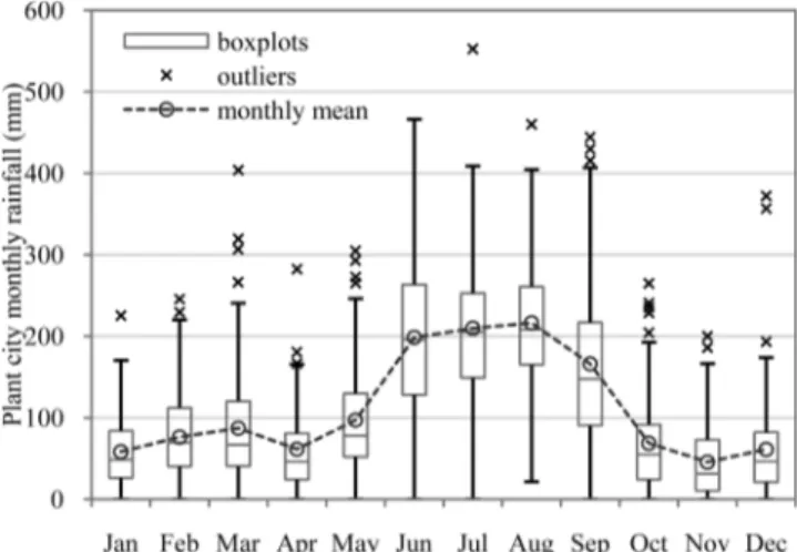
Preliminarily, monthly PC observation data were analyzed on a percentile basis. Fig. 2 shows mean rainfall totals for each calendar month as well as calendar monthly boxplots for rainfall totals. Mean rainfall totals exhibited a seasonal oscillatory pattern; more rainfall typically occurred in June

Fig. 2 Calendar monthly mean and boxplots of monthly total rainfall over the 102-year Plant City rainfall record

through September (wet season) than in other calendar months.

Boxplots showed that distributions of rainfall totals in each calendar month followed a seasonal pattern as well. Median rainfall totals followed the same seasonal oscillatory pattern as mean rainfall totals. Inter-quartile ranges, whiskers, and outliers all indicated that dry-month distributions had lower scatter and more skewness than wet season distributions.

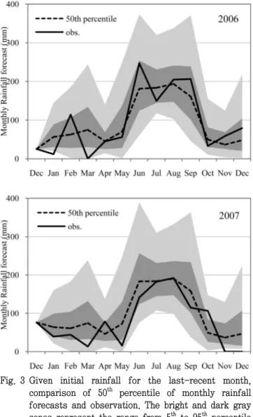
The assessment of the FMS forecasting methodology involves generating forecast output from a historical initial condition (December 2005 and December 2006) over a 1-year forecast period and comparing to actual monthly rainfall over that time period. Performance of the rainfall forecast model for 2006 and 2007 were evaluated by comparing several

Fig. 3 Given initial rainfall for the last-recent month, comparison of 50^th percentile of monthly rainfall forecasts and observation. The bright and dark gray zones represent the range from 5^th to 95^th percentile and from 25^th to 75^th percentile of 5,000 rainfall forecasts, respectively

percentiles of forecasts (i.e., 5^th, 25^th, 50^th, 75^th, and 95^th percentile) to the observations at the PC rain gage. Fig. 3 compares observed monthly rainfall to the rainfall forecasts generated by the FMS for 2006 and 2007. The results indicate that 50^th percentile of forecasts is well matched to the ob- served annual cycle of monthly rainfall in both years. Observed monthly rainfalls were within the 25^th and 75^th percentiles of the forecasts for almost months while several outliers were found especially in dry months. The outliers indicated that FMS would be limited in reproducing rainfall for extreme events, such as extreme drought, convective storms and hurricane seasons. The mean of forecasted 50^th percentile monthly rainfall over 2006 and 2007 were 3.6 in and 3.8 in, respectively while observed mean rainfall were 3.7 in and 3.0 in. That is, drought events during the dry season in 2007 were not reproduced by the current forecast system. This was likely because the rainfall forecasts were forced by initial conditions using observed data in the last-recent month and constructed using the statistics of the entire period of record.

It should be recognized that the model did not account for inter-annual cycling phenomena such as that associated with the El Niño-Southern Oscillation (ENSO). ENSO is known to have strong influences on rainfall in the study area, particularly during winter months (November-March) (Schmidt et al., 2001).

For future work, more detailed modeling structures could be defined to capture multi-year oscillation patterns, such as segmenting the historical record into El Niño/La Niña

“seasons” spanning multiple years and modeling each subset of the record separately. Additionally it was found that just 1-2 months of rainfall were influenced by the given initial condition and then the forecasts converged to simulation bounds. Currently, the possibility of improving the rainfall simulation using a three state (dry, normal, wet) Hidden Markov Model is being investigated. These seasonal models are expected to reproduce consistent dry or wet conditions.

2. Flow Forecast Results using Current Rainfall Forecast

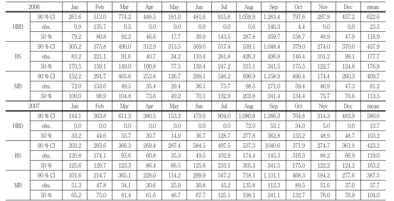
The results of the flow forecasts at the three streamflow stations (HRD, MB, and BS) were compared to observed streamflow in 2006 and 2007 to evaluate the flow predictions from the current model. Table 1 compares the 50^th percentile and the 90 % confidence interval (i.e., range between 5^th and 95^th percentile of flow forecasts) of flow forecasts using

Table 1 FMS flow forecast results for Hillsborough River Dam, Bell Shoal, and Morris Bridge stations using current rainfall forecast method for 2006 and 2007 (Unit: MGD, mega gallon/day)

2006 Jan Feb Mar Apr May Jun Jul Aug Sep Oct Nov Dec mean

HRD

90 % CI 261.6 513.0 774.2 448.5 181.0 481.6 915.8 1,059.9 1,283.4 797.6 297.9 457.2 622.6

obs. 0.9 135.7 0.5 0.0 0.0 0.0 0.0 0.6 140.3 4.4 0.0 0.0 23.5

50 % 79.2 80.8 92.2 46.6 17.7 39.9 143.5 287.8 359.7 158.7 48.9 47.9 116.9

BS

90 % CI 305.2 375.8 490.0 312.9 313.5 569.0 517.4 539.1 1,048.4 379.0 274.0 370.0 457.9

obs. 83.2 221.1 91.6 40.7 34.2 110.4 281.8 426.3 496.8 146.4 101.2 99.1 177.7

50 % 170.5 159.1 149.0 100.8 77.5 139.4 247.2 315.1 341.5 175.5 122.7 124.8 176.9

MB

90 % CI 152.2 291.7 465.6 253.8 126.7 299.1 546.2 696.9 1,158.9 490.4 174.4 260.3 409.7

obs. 72.0 153.6 49.5 35.4 29.4 36.1 75.7 98.5 271.0 59.4 46.9 47.3 81.2

50 % 100.0 98.9 104.8 73.6 49.2 70.1 132.9 203.8 241.4 134.4 75.7 76.6 113.5

2007 Jan Feb Mar Apr May Jun Jul Aug Sep Oct Nov Dec mean

HRD

90 % CI 144.1 363.8 611.3 380.5 153.3 479.9 904.0 1,080.8 1,286.3 764.8 314.3 483.9 580.6

obs. 0.0 0.0 0.0 0.0 0.0 0.0 0.0 72.0 53.1 34.0 5.0 0.0 13.7

50 % 33.2 44.6 55.7 30.7 14.9 36.7 128.7 277.8 362.8 155.2 48.9 48.7 103.2

BS

90 % CI 203.2 283.6 366.3 269.4 287.4 584.5 497.5 537.3 1040.6 371.9 274.7 361.9 423.2

obs. 120.8 174.1 93.6 60.8 35.3 49.5 102.9 174.4 145.3 316.3 88.2 66.9 119.0

50 % 125.6 129.7 123.3 86.4 66.5 125.6 233.1 305.3 341.5 175.0 122.2 124.2 163.2

MB

90 % CI 101.6 214.7 365.1 228.0 114.2 299.9 547.2 718.1 1,131.1 468.3 184.2 277.6 387.5

obs. 51.3 47.8 34.1 30.6 25.9 30.8 45.2 135.8 112.3 89.5 51.6 37.0 57.7

50 % 65.2 75.0 81.4 61.6 46.7 67.7 125.1 198.1 241.1 132.7 76.0 76.9 104.0

90 % CI: 90 % Confidence interval (Streamflow between 5 and 95 percentile predictions) obs.: Observed total monthly streamflow (MGD)

50 %: 50^th percentile of forecast streamflow

the rainfall forecasts to observed streamflow for 2006 and 2007. The results indicate that 50th percentile forecasts generally overestimated observed streamflow while the 90 % confidence interval encloses the observed monthly streamflow.

Note that monthly rainfall observations well conformed to 50^th percentile of rainfall forecasts. In particular, for the HRD station observed streamflow was reproduced within 5^th and 25^th percentile of forecasts (not shown). This was due to historical variability at this station is significantly high and it results in the wide range of forecasts. Additionally, it was found that the forecasts for each station tend to converge after several months, indicating the influence of the initial condition.

To assess the duration over which forecast bounds converge to simulation bounds, the differences between the annual cycles of the 50^th percentile of monthly forecasts in 2006 and 2007 for the three target stations were compared in Fig. 4a. Additionally standardized differences (i.e., (50^th percentile in 2006-50^th percentile in 2007)/ 50^th percentile in 2006) were calculated and compared in Fig. 4b. The results

indicate that initial conditions have influence on forecasted FMS flows over a period of 4-6 months, after which the standardized difference between forecasted and simulated results are less than 10 %. The flows at the BS and HRD station show convergence of forecast to simulation over approximately 6 months, while Morris Bridge forecasts con- verge over about 4 months. The number of months required for this convergence would imply the life of the forecast, or the duration of time through which the initial condition has influence over model results. These convergence assessments are qualitative and depend on how small a simulated-forecast deviation must be before convergence is assumed. Also, it is possible that convergence will vary depending on starting month. It should be noted that the time to convergence could vary depending on the initial month and station. The forecast from other starting months (e.g., a month of the wet season when the short-term temporal variability is significant) should be reexamined to address the time to convergence. Based on the results shown here, however, a 4-month cycle of forecast updating would seem reasonable.

(a) (b)

Fig. 4 (a) Difference and (b) standardized difference (i.e., monthly difference/simulation) between the 50^th percentile of 1-year monthly flow forecasts using current FMS rainfall forecast for 2006 and 2007

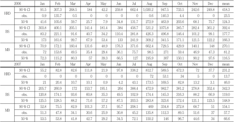
Table 2 FMS flow forecast results using the observed rainfall data for 2006 and 2007

2006 Jan Feb Mar Apr May Jun Jul Aug Sep Oct Nov Dec mean

HRD  

90 % CI 91.5 307.3 268.5 184 42.2 259.8 662.4 1,030.2 947.5 733.5 242.6 249.8 418.3

obs. 0.9 135.7 0.5 0 0 0 0 0.6 140.3 4.4 0 0 23.5

50 % 41.6 105.6 59.7 25.7 7.9 34.8 131.7 272.9 463.9 203.6 68.1 75.7 124.3

BS  

90 % CI 303.8 400.1 205.1 141.4 181.4 384 456.7 531.2 1075.8 385.7 282.4 361.2 392.4

obs. 83.2 221.1 91.6 40.7 34.2 110.4 281.8 426.3 496.8 146.4 101.2 99.1 177.7

50 % 173 161.6 99.7 67.9 53.4 133 241.9 309.2 341.5 171.1 121.5 122.2 166.3

MB  

90 % CI 70.9 172.1 160.4 131.6 48.9 176.3 371.6 662.4 729.5 429.9 140.1 148 270.1

obs. 72 153.6 49.5 35.4 29.4 36.1 75.7 98.5 271 59.4 46.9 47.3 81.2

50 % 72.3 115.2 80.3 57 39.3 66.5 127 195.9 307 150.1 90.2 97.6 116.5

2007 Jan Feb Mar Apr May Jun Jul Aug Sep Oct Nov Dec mean

HRD  

90 % CI 55.2 82.8 82.6 111.8 21.9 97.8 338.2 812.7 589.5 472.3 72 37.7 231.2

obs. 0 0 0 0 0 0 0 72 53.1 34 5 0 13.7

50 % 21 20.4 10.7 10.1 0.9 4.2 43.1 173.5 169.5 82.8 13.2 3.1 46.0

BS

90 % CI 205.7 260.9 172 153.7 195.1 264 388.4 472.9 982.7 381.2 278.8 352.4 342.3

obs. 120.8 174.1 93.6 60.8 35.3 49.5 102.9 174.4 145.3 316.3 88.2 66.9 119.0

50 % 125.5 128.5 88.2 71.6 57.2 87.5 203.5 283.8 323.6 172.4 121.1 123.5 148.9

MB  

90 % CI 52.8 75.5 82.9 101.3 37.1 95.7 208.1 469 334.8 272.8 68.7 51 154.1

obs. 51.3 47.8 34.1 30.6 25.9 30.8 45.2 135.8 112.3 89.5 51.6 37 57.7

50 % 53.5 53.8 41.8 42.7 29.2 34.5 72.1 150.2 146 96.7 44.6 34 66.6

90 % CI: 90 % Confidence interval (Streamflow between 5 and 95 percentile predictions) obs.: Observed total monthly streamflow (MGD)

50 %: 50^th percentile of forecast streamflow

These results are quite comparable to those that Tampa Bay Water previously reported while developing the model (Hazen and Sawyer, 2005). They ran the model for 2 con- secutive years from April 2003 to March 2005. Then the results were split into two periods (i.e., April 2003-March

2004 and April 2004-March 2005) and compared monthly forecasts assuming the simulations for the second period contain no effects of the initial condition. They concluded that it takes 3 to 6 months to converge and the results may vary with the stations.

3. Flow Forecast Results using the Observed Rainfall Data

The flow predictions were then repeated using the actual observed rainfall instead of the time series model forecasted rainfall, in each streamflow time series model. Table 2 com- pares the 50^th percentile and the 90 % confidence interval of flow forecasts using the monthly rainfall observation to observed streamflow for 2006 and 2007. The results indicate that the 50^th percentile of streamflow forecasts at the HRD station still overestimated the observation while the monthly streamflow observations for the BS and MB station were reasonably reproduced by the 50^th percentile forecast. The reason for this is that flow at HRD is regulated and the operation of the small reservoir may not be totally captured by the modeling effort. Another important factor is that there may be groundwater interaction at TBC that is not explicitly captured by the models. Most importantly, analysis of these results show that the 90 % confidence interval band for streamflow predictions was reduced by 14 %, 32 %, and 34 % for the BS, MB, and HRD station, respectively when using the observed rainfall data in 2006 and 19 %, 61 %, and 60 % for each station in 2007. These results indicate the potential for improving model performance if better rainfall forecasts can be incorporated into the FMS system. In addition, the present analysis has also highlights the maximum improvement that one can expect even with the perfect rainfall knowledge.

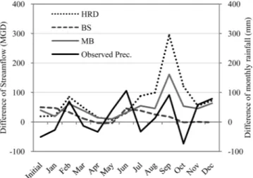
Fig. 5 Difference between 50^th percentiles of the 1-year monthly flow forecasts using the observed rainfall data and observed monthly rainfall for 2006 and 2007

Fig. 5 compares the differences between 50^th percentile flow forecasts using the observed rainfall data in 2006 and 2007 for each station. Also shown in this figure is the di- fference between the observed monthly rainfall amounts for 2006 and 2007, which were used to simulate the flow forecasts as the perfect rainfall forecast scenario. The results show that flow forecast convergences were a result of the rainfall forecast (see Fig. 4a). The divergences of monthly flow forecasts were largest during the wet season from July to October based on differences in forcing input (i.e., monthly rainfall observation in this case). This finding implies the vulnerability of flow forecast during the wet season, to some extent, even when the rainfall scenario is accurately developed.

V. SUMMARY

This paper introduced the flow forecast modeling system that a water management agency in west central Florida, Tampa Bay Water has been operated to forecast monthly rainfall and streamflow in the Tampa Bay region, Florida.

We evaluated current 1-year monthly rainfall forecasts and flow forecasts and actual observations to investigate the benefits of incorporating rainfall forecasts into monthly flow forecast.

Results for rainfall forecasts showed that the observed annual cycle of monthly rainfall was accurately reproduced by the 50^th percentile of forecasts. While observed monthly rainfall was within the 25^th and 75^th percentile of forecasts for most months, several outliers were found during the dry months especially in the dry year of 2007. The flow forecast results for the three streamflow stations (HRD, MB, and BS) indicated that while the 90 % confidence interval mostly covers the observed monthly streamflow, the 50^th percentile forecast generally overestimated observed streamflow. Es- pecially for HRD station, observed streamflow was reproduced within 5^th and 25^th percentile of forecasts while monthly rainfall observations closely followed the 50^th percentile of rainfall forecasts. This was due to the historical variability at the station was significantly high and it resulted in a wide range of forecasts. Additionally, it was found that the forecasts for each station tend to converge after several months as the influence of the initial condition diminished.

The forecast period to converge to simulation bounds was estimated by comparing the forecast results for 2006 and 2007. We found that initial conditions have influence on forecasts during the first 4-6 months, indicating that FMS forecasts should be updated at least every 4-6 months.

That is, knowledge of initial condition (i.e., monthly flow observation in the last-recent month) provided no fore- knowledge of the flows after 4-6 months of simulation.

Based on the experimental flow forecasts using the observed rainfall data, we found that the 90 % confidence interval band for flow predictions was significantly reduced for all stations.

This result evidently shows that accurate short-term rainfall forecasts could reduce the range of streamflow forecasts and improve forecast skill compared to employing the stochastic rainfall forecasts. We expect that the framework employed in this study using available observations could be used to investigate the applicability of existing hydrological and water management modeling system for use of state- of-the-art climate forecasts.

REFERENCES

1. Asefa, T., N. Wanakule, and A. Adams, 2007. Field- scale applicability of three types of Artificial Neural Networks to predict groundwater levels.

Journal of American Water Resources Association

JAWRA

1-12. DOI: 10.1111/j.1752-1688.2007.00107.

2. Brath, A., P. Burlando, and R. Rosso, 1988. Sensitivity analysis of real-time flood forecasting to on-line rainfall predictions. Selected paper from the workshop on Natural Disasters in European-Mediterranean Countries, Perugia, Italy, pp. 469-488.

3. Clayton, J., T. Asefa, A. Adams, and A. Anderson, 2010.

Interannual-to-Daily Multiscale Stream Flow Models with Climate Effects to Simulate Surface Water Supply Availability, In: Innovations in Watershed Management under Land Use and Climate Change.

Proceeding of the 2010 Watershed Management Conference

4. Florida Division of Forestry, 2005. Florida’s Forest Resources Plan Setting the Course for 2030: 1. Present

Condition of Florida’s Forest Resources, retrieved: January 10, 2010, from: http://www.fl-dof.com/plans_support/ps_

pdfs/FlForestResourcesActionPlan12_2005.pdf.

5. French, M. N., W. F. Krajewski, and R. R. Cuykendall, 1992. Rainfall forecasting in space and time using a neural network.

Journal of Hydrology

6. Hazen and Sawyer, 2005. Tampa Bay Water Future Need Analysis: A modeling system for stochastic simulation of permit flows for the Enhanced Surface Water System.

7. Hwang, S., W. Graham, J. L. Hernández, C. Martinez, J.

W. Jones, and A. Adams, 2011. Quantitative Spatiotemporal Evaluation of Dynamically Downscaled MM5 Precipitation Predictions over the Tampa Bay Region, Florida.

Journal of Hydrometeorology

8. Kişi, O., 2007. Streamflow forecast using different artificial neural network algirithms.

Journal of Hydrologic Engineering

9. Lee, S. J., C. S. Jeong, J. C. Kim, and M. H. Hwang, 2011. Long-term Streamflow Prediction Using ESP and RDAPS Model.

Journal of Korea Water Resources Association

10. Schmidt, N., E. K. Lipp, J. B. Rose, and M. E. Luther, 2001. ENSO Influences on Seasonal Rainfall and River Discharge in Florida.

Journal of Climate

11. Schmidt, N., M.E. Luther, and R. Johns, 2004: Climate Variability and Estuarine Water Resources: A Case Study from Tampa Bay, Florida. Coastal Management 32: 101-116.

12. Southwest Florida Water Management District, 2012.

2010 Estimated Water Use In the Southwest Florida Water Management District. This report is available on the Internet at: http://www.swfwmd.state.fl.us/

13. Tampa Bay Water, 2011. Optimized Regional Operations Plan (OROP): Tampa Bay Water Annual report, 2011.

Submitted to Southwest Florida Water Management District.

14. Toth, E., A. Brath, and A. Montanari, 2000. Comparison of short-term rainfall prediction models for real-time flood forecasting.

Journal of Hydrology